Embedding Models and Retrieval Quality
The gateway controls how fast your system moves. The embedding model controls whether it moves in the right direction.
In an agentic system, this distinction matters more than most teams realize. If your gateway is slow, users wait. If your embeddings are wrong, the system confidently walks down the wrong path. And unlike latency, which is visible and measurable, retrieval errors are silent. They don’t throw exceptions. They don’t trip alerts. They simply corrupt the state on which every downstream decision depends.
A useful way to think about this is to treat retrieval as the “perception layer” of your system. Just as a self-driving car depends on correctly identifying lanes and obstacles before planning a path, your agent depends on retrieving the right context before generating, reasoning, or acting. If perception is wrong, planning becomes irrelevant. The system is solving the wrong problem perfectly.
Retrieval quality is a system property, not a model score
Most teams approach embedding model selection as a leaderboard problem. They compare MTEB scores, pick a top-ranked model, and move on. That works for demos. It fails in production.
Retrieval quality is not a property of the embedding model alone. It is a property of the interaction between your corpus, your query distribution, your chunking strategy, and your ranking behavior under ambiguity. The embedding model sits in the middle of this interaction - it is a compression function that maps language into a space where relevance becomes distance. The problem is that relevance is not universal. It is defined by your system.
Two documents can be equally similar to a query in a semantic sense and still differ completely in usefulness. One might be current, authoritative, and specific. The other might be outdated, generic, or structurally similar but contextually wrong. An embedding model that collapses this distinction is not bad in a general sense - it is misaligned with your system's notion of relevance. That mismatch is where most production retrieval issues originate.
Why MTEB is a filter, not a decision
The Massive Text Embedding Benchmark covers 56 datasets across 8 task types: retrieval, clustering, classification, semantic textual similarity, reranking, and others. The overall score is an average across all of them. A model that tops the overall leaderboard may be optimized for semantic textual similarity or classification - tasks that share mathematical structure with retrieval but are not retrieval. For RAG workloads, the retrieval-specific MTEB scores are the relevant signal. A model ranked 8th overall but 2nd on retrieval tasks is a better candidate than one ranked 1st overall but 5th on retrieval.
Even retrieval-specific MTEB scores are measured on a fixed set of benchmark corpora - Wikipedia, scientific papers, legal documents, news articles. A model that achieves 0.72 nDCG@10 on BEIR may achieve 0.51 on your internal enterprise knowledge base if your documents use specialized terminology, domain-specific acronyms, or writing styles not well-represented in the benchmark. This is not a flaw in the benchmark. It is distribution shift - the same gap that makes offline ML evaluation an approximation of production behavior.
Use MTEB to filter out clearly weak candidates. Validate every serious candidate against your own corpus before committing. The sections that follow describe exactly how to do that.
Hard negatives are where models actually fail
If synthetic queries define the problem space, hard negatives define the difficulty. Without hard negatives, almost every modern embedding model looks good. Distinguishing between unrelated topics is a solved problem. The production challenge is distinguishing documents that are close in meaning but different in outcome.
Consider a query about KV cache memory usage in an LLM serving system. A typical corpus contains:
- a document describing KV cache scaling behavior
- a document describing model weight memory layout
- a document describing context length limits
All three are semantically related. Only one answers the question. A weak model retrieves all three at similar similarity scores. A strong model ranks the correct one first - because it has learned to separate documents that are topically similar but differ in the specific aspect the query targets.
Hard negatives simulate one of the most important production retrieval conditions: semantically similar documents that differ in answer relevance. They are documents that are topically similar, structurally similar, and often share identical terminology with the relevant document - but do not answer the query. Without them, your evaluation measures separation between distant clusters. With them, it measures ordering within a dense cluster. Production retrieval lives entirely in the second regime.
This is the closest offline approximation of real-world retrieval ambiguity - and it is the reason that a model's hard-negative performance predicts production behavior far better than its headline MTEB score.
Recall defines the ceiling of your system
There is a hard constraint in retrieval-augmented systems: the system cannot produce a correct answer based on information it never retrieved.
If the relevant document is not among the top-k results, it is invisible to everything downstream. No reranker can promote it. No LLM can infer it reliably. No agent can reason about it. The system is operating under incomplete information, and everything that follows is a best-effort approximation.
You can think of retrieval as assembling the pieces of a puzzle. Recall determines whether the necessary pieces are even on the table. Precision determines how cleanly they are arranged. You can fix a messy arrangement. You cannot fix missing pieces.
In practice, recall improvements compound nonlinearly. As recall climbs, system quality improves rapidly up to a point, then plateaus. When critical documents start getting excluded from the candidate set, system quality degrades sharply - not gradually. It feels like a phase transition: the system suddenly becomes unreliable rather than progressively worse. This is why teams that optimize precision first and recall second are often surprised by production failures that offline metrics did not predict.
Recall@k measures this directly - of all truly relevant documents in your corpus, how many appear in the top-k retrieved results:
Recall@k = (relevant documents in top-k) / (total relevant documents in corpus)

Example:
  Total relevant documents for query: 8
  Relevant documents in top-10: 6
  Recall@10 = 6/8 = 0.75
nDCG@10 (Normalized Discounted Cumulative Gain) rewards both relevance and rank position. A relevant document at position 1 contributes more than one at position 10. Use nDCG when you care about ordering - particularly for RAG without a downstream reranker, where top-ranked chunks are weighted more heavily in context assembly.
MRR (Mean Reciprocal Rank) focuses on where the first relevant result appears. Useful for narrow retrieval tasks with one correct answer - policy lookups, runbooks, specific fact retrieval. Less useful for broad knowledge questions where multiple relevant documents exist.
Why rerankers cannot rescue poor retrieval
A common architectural response to weak retrieval is to add a reranker. This is often framed as a safety net. In practice, it is more like a filter applied to whatever the retrieval stage provides - it can only reorder what it sees.
If the correct document is not in the candidate set, the reranker has nothing to work with. It cannot search beyond the inputs it receives. It cannot invent missing context. You can compensate by increasing k - expanding the candidate set so that recall improves - but this introduces a cascade of secondary problems. Larger candidate sets increase reranker latency, increase LLM context token costs, and increase the signal-to-noise ratio that every downstream component must manage. At scale, what starts as a modeling weakness becomes an infrastructure tax that grows with every query.
This leads to a clear design principle: optimize retrieval for recall first, address precision downstream. The reranker is for ordering a good candidate set - not for rescuing a poor one.
The illusion of semantic similarity
One of the more subtle traps in embedding systems is the belief that high cosine similarity implies correct retrieval. It does not.
Similarity measures whether two pieces of text are related. Retrieval requires deciding which related piece is the correct one - under constraints that are often invisible to a general-purpose embedding model.
A useful analogy: imagine navigating to your house using a heatmap that highlights areas "similar to your neighborhood" - same architecture, same street layout, same general environment. The heatmap will guide you to places that feel right. But unless it encodes your specific address, it will not take you home. Embedding models optimized for general semantic similarity behave in exactly this way. They cluster related content effectively but do not always enforce the specific distinctions that make one document the right answer and another merely relevant.
Consider a query "What is our SLA for Tier 1 incidents?" in an enterprise knowledge base. A model optimized for semantic similarity will score this highly against any document mentioning SLAs, incidents, and response times - including a document describing competitor SLAs, a historical document with outdated figures, and a template with placeholder values. These documents are semantically similar. None of them is the right answer.
Retrieval quality requires the model to rank the authoritative, current, specific document above the merely similar ones. This is a different capability from semantic similarity, and it is the one that determines production usefulness.
This becomes particularly acute in enterprise systems where many documents are variations of the same theme: policies have versions, runbooks have environments, designs have iterations, templates coexist with instantiated documents. The model must not only understand similarity - it must enforce distinctions that are invisible at a purely semantic level. When it fails, the system retrieves documents that are technically relevant but operationally wrong. These are the hardest errors to detect, because they appear plausible.
Domain adaptation is about ranking, not understanding
By the time you are working with modern embedding models, basic language understanding is not the bottleneck. The model already knows what "SLA" means. It understands incidents, policies, and metrics. What it does not know is how your organization prioritizes them.
Fine-tuning or adapting an embedding model in this context is not about teaching it new language. It is about teaching it how to order documents correctly under your system's constraints - shaping the geometry of the embedding space so that:
- authoritative documents rank above similar but outdated variants
- version-specific documents rank above templates and examples
- documents that are subtly but operationally different become separable
This is why domain-adapted models often outperform general models even when their benchmark scores are comparable. The difference is not representational capacity. It is alignment with your relevance structure. A general model understands your domain. A fine-tuned model understands your domain's relevance ordering.
Agentic systems amplify retrieval errors
In a standard RAG pipeline, a retrieval error is typically contained within a single response. The model produces a slightly incorrect answer, and the error ends there.
Agentic systems behave differently. They introduce state, iteration, and feedback loops that transform a single retrieval error into a trajectory failure.
An incorrect retrieval early in an agent's execution influences the plan it constructs, the tools it calls, the intermediate results it stores, and the subsequent queries it generates. The system begins to build on incorrect assumptions. Each step reinforces the previous one. The agent drifts further from the correct solution - often with increasing confidence, because the subsequent reasoning is internally consistent even when the premise is wrong.
Think of retrieval as the perception layer of the agent. A self-driving car that misidentifies a lane boundary does not just make one wrong steering decision - it continues planning and executing from a corrupted map of reality. Downstream path planning, speed control, and obstacle avoidance all operate correctly on incorrect inputs. The system is solving the wrong problem perfectly.
Retrieval errors in agentic systems work the same way. The agent's reasoning capability is not in question. Its grounding is. A retrieval error at turn 1 that goes undetected propagates into every subsequent turn, and the further the agent progresses, the more expensive the correction becomes - both in tokens and in the downstream actions that may have already been taken.
This makes retrieval quality foundational in agentic systems in a way it is not in single-turn RAG. Every downstream investment - prompt engineering, tool design, multi-step orchestration, guardrails - depends on the retrieval foundation being solid. If retrieval is weak, every other investment becomes an attempt to stabilize a system that is working from incomplete or incorrect information.
The production perspective
At this level, selecting an embedding model is not about choosing the one with the highest score. It is about designing a system that:
- maintains high recall under your specific query distribution
- preserves critical distinctions in ranking when documents are semantically close
- does not rely on downstream components to compensate for upstream retrieval gaps
- degrades gracefully when query distribution shifts, rather than failing silently
If retrieval is weak, every other optimization - reranking, prompt engineering, agent orchestration - becomes a stabilization effort rather than a performance improvement. You are not building capability. You are managing a deficit.
Stability, at scale, always begins with getting retrieval right. The sections that follow give you the tools to do that: how to measure retrieval quality on your own data, how to select and adapt models correctly, and how to detect when retrieval quality is degrading in production before users do.
Benchmarking on your own data
Before you select a model, you need an evaluation instrument. This is not optional - it is the step that separates a model selection decision that holds up in production from one that looked good on paper.
The instrument is a domain-specific evaluation set: a collection of (query, relevant document, hard negative documents) triplets drawn from your actual corpus. Every serious model selection decision should be made against this, not against MTEB.
Building a domain-specific eval set without labeled data
Human-labeled (query, relevant document) pairs at scale are expensive, slow, and often inconsistent across annotators. The practical alternative for most production teams is synthetic query generation - using a frontier LLM to generate realistic queries for a sample of your documents, then treating each (generated query, source document) pair as a positive example.
python
# For each document chunk in your evaluation sample:
prompt = f"""
Generate 3 realistic questions that this document passage would answer.
Questions should reflect how a user would actually phrase them -
not document titles, not keyword searches.
Questions should vary in phrasing and specificity.
Return only the questions, one per line.

Document:
{document_chunk}
"""
# Each (question, document_chunk) pair is a positive example in your eval set.
# The document_chunk is the ground truth relevant document for that question.
Two things determine the quality of this eval set more than anything else.
LLM quality for generation. A weak model generates questions that are too literal - paraphrases of document headings rather than the ambiguous, paraphrastic queries your users actually ask. Use a frontier model. The cost of generating an eval set is a one-time investment; the cost of selecting the wrong embedding model and reindexing at scale is not.
Document sampling strategy. Your eval set is only as representative as the documents you sample from. The failure mode here is sampling from your most common document type because it is easiest - and then discovering that the selected model performs poorly on your long-tail document types that happen to drive the most complex queries. Sample across the full range: topics, document types, writing styles, ages, and sources. A 500-document sample that is representative outperforms a 5,000-document sample that is not.
Hard negative mining
Synthetic queries give you positive pairs - a question and the document that answers it. Hard negatives give you the difficulty signal that separates a useful eval set from a trivial one.
The mechanism works in three steps, and understanding all three is important before looking at the code.
Step 1 - Frontier LLM establishes ground truth. For each document chunk, a frontier model (Claude, Gemini) generates realistic queries that the document answers. Each (query, document_chunk) pair becomes a positive example. The frontier LLM is acting as the judge of relevance: "this document is the correct answer to this question." You now have ground truth - a mapping from query to correct document ID.
Step 2 - Your baseline embedding model reveals its confusion. Take each query from Step 1 and run it through your baseline embedding model. Do a vector search against your full corpus. The model returns the top-k most similar documents - ranked by embedding similarity, not by whether they actually answer the query. The correct document may appear at rank 1, rank 5, or not at all. The documents ranked above the correct answer are the ones the embedding model found more similar.
Step 3 - The disagreement is your hard negative set. You know the correct answer from Step 1. You know what the embedding model retrieved from Step 2. Any document that ranked high in the vector search but is not the correct answer is a hard negative - a document the embedding model confused with the right answer. The filter is a simple ID comparison: everything in the top-k results that does not match the ground truth document ID.
def build_eval_set_with_hard_negatives(
    corpus_chunks,
    baseline_model,
    frontier_llm,
    sample_size=500
):
    eval_set = []

    # Step 1: Generate ground truth positives using frontier LLM
    for chunk in sample(corpus_chunks, sample_size):
        queries = frontier_llm.generate(f"""
            Generate 3 realistic questions this document passage would answer.
            Phrase them as a user would ask - not as document titles.
            Vary phrasing and specificity across the 3 questions.
            Return only the questions, one per line.

            Document: {chunk.text}
        """)

        for query in queries:
            # Ground truth: this chunk IS the correct answer to this query
            positive_doc_id = chunk.id

            # Step 2: Run query through baseline embedding model
            query_embedding = baseline_model.embed(query)
            top_k_results = vector_search(query_embedding, corpus_index, k=20)
            # top_k_results is an ordered list of document IDs by similarity score

            # Step 3: Hard negatives = high-ranking results that are NOT the answer
            # Simple ID comparison - no semantic matching needed
            hard_negatives = [
                doc_id for doc_id in top_k_results
                if doc_id != positive_doc_id  # exclude the correct answer
            ][:5]  # top 5 confusions are enough; more dilutes the signal

            eval_set.append({
                "query":          query,
                "positive":       positive_doc_id,
                "hard_negatives": hard_negatives,
            })

    return eval_set
The hard negatives here are not randomly sampled documents. They are the specific documents your baseline embedding model gets confused by - the ones it ranked higher than the correct answer. A candidate model that correctly ranks the positive document above these hard negatives has demonstrated exactly the discriminative capacity that production retrieval requires: not just finding relevant documents, but ranking them correctly against the specific confusions that will actually occur in your corpus.
This is also why using a strong baseline model for hard negative mining produces better hard negatives than using a weak one. A stronger baseline returns more semantically similar documents in its top-k - which means its confusions are harder confusions, and the resulting eval set is a more stringent test.
One calibration note: a well-constructed eval set has 3-5 hard negatives per query. More than 5 dilutes the difficulty signal - the discriminative value comes from genuinely confusing near-misses, not from adding easier negatives that pad the set.
Running the evaluation
With queries, positive documents, and hard negatives in place, the evaluation protocol produces the three signals you need to make a model selection decision: retrieval quality, latency, and cost. All three matter - a model with excellent recall but 800ms P95 embedding latency may not fit your SLO, and a model with strong quality at prohibitive cost may not fit your budget at production volume.
import time

# ground_truth is a list of (query, correct_document_id) pairs -
# the output of your eval set construction from the previous section.
# Each entry says: "for this query, THIS is the document that answers it."
#
# Example:
# ground_truth = [
#   ("What is our SLA for Tier 1 incidents?", "doc_policy_sla_v3"),
#   ("How do I rotate an API key?",           "doc_runbook_api_keys"),
#   ("What changed in the Q2 pricing model?", "doc_pricing_q2_2026"),
# ]
#
# eval_queries is just the list of queries extracted from ground_truth:
# eval_queries = [query for query, _ in ground_truth]

results = {}

for model in candidate_models:

    # Batch embed all queries at once - never one at a time.
    # One-by-one embedding is 10-30x slower than batched, which makes
    # latency measurements meaningless and eval runs impractically slow.
    query_embeddings = model.embed_batch(eval_queries)

    recalls, latencies = [], []

    # Zip pairs each embedded query back with its known correct document ID.
    # query_emb:       the vector representation of the query
    # relevant_doc_id: the document that should appear in the top-k results
    for query_emb, (_, relevant_doc_id) in zip(query_embeddings, ground_truth):

        start = time.perf_counter()

        # Search against the full corpus index - not just the eval documents.
        # Recall behaves differently at 500 documents vs 5 million.
        # ANN index structure, distance distributions, and hard negative
        # density all change at scale. Evaluate under production conditions.
        top_k_doc_ids = vector_search(query_emb, full_corpus_index, k=10)
        # top_k_doc_ids is an ordered list of document IDs by similarity:
        # e.g. ["doc_abc", "doc_xyz", "doc_policy_sla_v3", ...]

        latencies.append((time.perf_counter() - start) * 1000)  # ms

        # Binary recall@10: is the correct document anywhere in the top-10?
        # 1.0 = yes (retrieved), 0.0 = no (missed)
        # Binary is appropriate here - the question is presence, not position.
        # Use nDCG if you care about whether the correct doc ranked 1st vs 8th.
        recalls.append(1.0 if relevant_doc_id in top_k_doc_ids else 0.0)

    results[model.name] = {
        "recall@10":          sum(recalls) / len(recalls),
        "latency_p50_ms":     sorted(latencies)[len(latencies) // 2],
        "latency_p95_ms":     sorted(latencies)[int(len(latencies) * 0.95)],
        # P95 not P50 - your SLO is defined by the tail, not the median.
        # A model with low P50 but a heavy P95 tail will breach your SLO
        # under the bursty traffic patterns typical of enterprise workloads.
        "cost_per_1M_tokens": model.embedding_cost_per_1M_tokens,
    }
Interpreting the results. The delta between a model's MTEB retrieval score and its Recall@10 on your domain eval set is your distribution shift signal. A model that drops more than 15 percentage points - say 0.68 MTEB to 0.51 on your corpus - has a meaningful mismatch: your documents are out-of-distribution for that model. This narrows your candidate set to models that are better matched to your domain, or strong candidates for domain adaptation covered in Section 4.
When comparing two models where one has higher recall but higher latency, the decision depends on where you sit on the retrieval-latency tradeoff for your specific SLO. There is no universal answer - but a model that wins on both recall and latency across your eval set is the clear choice, and one that loses on both should be eliminated regardless of MTEB ranking.
A/B testing models in production without full reindexing
Offline evaluation against your domain eval set tells you how a candidate model performs on a fixed set of queries. Before you can act on those results, you need to understand what switching embedding models actually requires - and why it is not a simple swap.
What a vector index is and why it has to be rebuilt
Your retrieval system does not compare a query vector against every document vector at query time - that would be linear scan at millions of documents and take seconds per query. Instead, your corpus documents are pre-embedded and organized into a vector index: a data structure (HNSW, IVF, and others - covered in depth in Chapter 3) that lets you find the nearest document vectors to a query vector in milliseconds.
That index is built from the embeddings produced by your current embedding model. When you switch to a new embedding model, every document in your corpus needs to be re-embedded from scratch - because the new model produces vectors in a completely different geometric space than the old one. Old vectors and new vectors are not comparable. You cannot run a partial migration where half your documents use the old model and half use the new one. The entire index must be rebuilt before the new model can serve production traffic.
For a corpus of 10 million documents, this reindexing can take hours of compute and significant cost. It is not a decision you want to make based on offline eval results alone.
Shadow indexing: production evidence before commitment
Shadow indexing lets you build the candidate model's index in parallel - while your current index continues serving users normally - and route a sample of real production queries to both indexes simultaneously. Users only ever see results from the current index. The candidate index results are logged and compared offline.
Incoming production query
        │
        ▼
Current index (old model) ──────────────────────► Return results to user
        │                                          (unchanged, zero latency impact)
        │  async fork - sampled at configured rate
        ▼
Candidate index (new model) ──► Log {query, retrieved_doc_ids, scores, latency}
                                 ──► Offline comparison queue
The shadow path must be strictly non-blocking. If the candidate index lookup can delay the primary response under any condition - shared thread pools, shared connection limits, resource contention under load - you have introduced production latency risk in the name of evaluation. Implement the shadow fork as a fire-and-forget background task dispatched after the primary results are returned to the user.
What to compare from shadow logs
Downstream quality signals are the most direct evidence of retrieval quality difference. If you have user feedback - clicks on retrieved results, explicit thumbs up/down ratings, follow-up queries that suggest the first answer was wrong - compare these between queries served from the current index and those shadowed to the candidate index. A candidate model that shows measurably better downstream quality signals in shadow has production evidence of improvement that no offline eval can match.
Rank correlation tells you whether the candidate model is retrieving the same documents in a different order, or genuinely different documents. High rank correlation with improved position for known-relevant documents suggests a quality improvement. Low rank correlation - substantially different document sets - requires deeper investigation before any production commitment.
Score distribution shift is subtle but important. If the candidate model's similarity scores are systematically lower than the current model's for the same queries, downstream components that use score thresholds - filtering out results below 0.7 similarity, for example - will silently reject more results than they used to. A score distribution shift that is not caught before cutover can break downstream filtering without any visible error.
Shadow indexing is the bridge between offline evaluation and production commitment. A candidate model that wins on your domain eval set and shows positive signals in shadow has earned the full reindex investment. A model that wins offline but shows neutral or negative signals in shadow has revealed a gap between your eval set and your actual production query distribution - which is valuable information that should drive eval set expansion before any model change is made.
Model selection framework
The right model for your system is determined by your constraints, not the leaderboard. Work through these decisions in order.
Dense vs. sparse retrieval - and why the distinction matters
Before selecting an embedding model, you need to make an architectural decision about how retrieval works in your system. This is the choice between dense retrieval, sparse retrieval, and hybrid combinations of both. These terms have nothing to do with model architecture, MoE routing, or parameter sparsity - they describe how documents and queries are represented for the purpose of finding matches.
Dense retrieval converts every document and every query into a fixed-size vector - a list of floating-point numbers - using a neural embedding model. Similarity between a query and a document is the geometric distance between their vectors in that high-dimensional space. The representation is called "dense" because every dimension carries information - no zeros, every number contributes to the meaning.
Sparse retrieval represents documents as term-frequency vectors - essentially a count of how often each word in the vocabulary appears in a document. For a vocabulary of 50,000 words, a document that uses only 200 of them has a vector with 49,800 zeros. The representation is "sparse" because most dimensions are zero. BM25 - which you may know from Elasticsearch or Lucene - is the most widely used sparse retrieval algorithm. It scores documents based on term overlap with the query, weighted by how rare each term is across the corpus.
A useful way to think about the difference: dense retrieval understands meaning, sparse retrieval understands words.
Imagine asking "What are the side effects of ibuprofen?" Dense retrieval understands that "adverse reactions," "contraindications," and "what happens if I take too much" are all semantically related and will surface relevant documents even if they use different phrasing. Sparse retrieval will surface documents that contain the exact word "ibuprofen" - which is what you want if you're looking for a specific drug identifier like "ibuprofen 400mg tablet ref-7823," but not if you want conceptual information about the drug class.
Now reverse the scenario. You're searching for "CVE-2024-29943" - a specific security vulnerability identifier. Dense retrieval will surface semantically related security documents. Sparse retrieval will find the exact document that mentions that specific CVE number. For exact identifiers, sparse wins decisively.
This asymmetry - dense handles meaning, sparse handles exact terms - defines when each approach fails and when hybrid is necessary.
When dense fails and when sparse fails
Dense retrieval fails on:
- Exact identifiers: product codes, CVE numbers, RFC numbers, ticket IDs, API version strings
- Rare proper nouns: person names, company names, internal codenames that the embedding model has not seen at scale
- Queries where the exact wording matters more than the concept - "is this covered under clause 4.2.1(b)?" requires finding clause 4.2.1(b), not semantically similar clauses
Sparse retrieval fails on:
- Paraphrastic queries: "How do I reset my password?" vs "What's the process to change my credentials?" - different words, same intent, sparse retrieval treats them as different queries
- Concept-level queries where the user doesn't know the exact terminology - "how do I make my model faster?" may not contain the terms "quantization," "batching," or "KV cache" even though those are the relevant documents
- Cross-lingual retrieval: a query in Spanish will not match an English document even if they mean the same thing
For most enterprise RAG deployments, your query distribution contains both types. Users who know the exact term they want, and users who are describing a concept. This is where hybrid retrieval earns its place.
Hybrid retrieval and the RRF merge
Hybrid retrieval runs both a dense ANN search and a sparse index lookup against the same query, then merges the two ranked lists into a single result. The most common merge strategy is Reciprocal Rank Fusion (RRF):
rrf_score(doc) = 1/(k + rank_dense) + 1/(k + rank_sparse)
A document that ranked 2nd in dense search and 5th in sparse search scores:
rrf_score = 1/(60+2) + 1/(60+5) = 0.0161 + 0.0154 = 0.0315
A document that ranked 1st in dense but didn't appear in sparse at all scores:
rrf_score = 1/(60+1) + 0 = 0.0164
The document with agreement across both systems - even at lower individual ranks - often scores higher than one that dominated a single system. This is the intuition behind RRF: documents that are relevant from multiple retrieval perspectives are more likely to be genuinely relevant.
The constant k (typically 60) controls how sensitive the score is to rank position differences. Higher k smooths the blend - rank 2 and rank 10 contribute similar scores. Lower k amplifies differences - rank 2 contributes substantially more than rank 10. Start with k=60, the value established in the original RRF paper, and tune only if you have clear evidence that rank position should dominate the merge.
The latency tax is real and must be measured. Hybrid retrieval runs two passes instead of one - a dense ANN search and a sparse index lookup - then merges results. At query volume, this adds 20-40ms of retrieval latency depending on index size and hardware. For latency-sensitive workloads, measure the actual cost on your infrastructure before committing. For workloads where better recall on exact-match queries justifies slightly higher latency, hybrid is almost always worth it.
Choose dense-only when: your query distribution is primarily paraphrastic, your latency SLO is tight, and your corpus does not contain documents where exact keyword matching is critical.
Choose hybrid when: your corpus contains specialized terminology, product codes, version strings, proper names, or technical identifiers - and your query distribution mixes conceptual and keyword-style queries. This describes most enterprise RAG deployments.
Model selection decision framework
Specific model recommendations go stale faster than any other content in this handbook - the embedding model landscape changes quarterly. What doesn't change is the set of constraints that determine which models are viable for your system. Work through these in order; each one eliminates candidates before you run your domain benchmarks.
1. MULTILINGUAL REQUIREMENTS
   Do your users query in multiple languages, or does your corpus
   contain documents in multiple languages?

   YES → Narrow to models with strong multilingual MTEB retrieval scores.
         Verify the specific languages you need are well-represented in
         the model's training data - multilingual coverage varies widely.
   NO  → English-only models are viable; typically stronger on English tasks.

2. DEPLOYMENT MODEL (data residency, licensing, cost at scale)
   Must you self-host? (regulatory, data residency, or cost reasons)

   YES → Narrow to open-weight models with commercial-use licenses.
         Verify license terms explicitly - some models prohibit commercial use
         or fine-tuning. Read the license, not just the marketing page.
   NO  → Managed APIs are viable. Factor in: no infrastructure overhead,
         but you accept vendor dependency, pricing changes, and API rate limits.

3. DOCUMENT CONTEXT LENGTH
   What is the P95 token length of your documents after chunking?

   UNDER 512 tokens:   most models handle this well
   512 - 2,048 tokens: verify the model's stated context window
   OVER 2,048 tokens:  narrow to models with long-context training support.
                       Context window and training context length differ -
                       a model can accept 8K tokens but degrade on long inputs
                       if it was not trained on long documents.

4. MRL DIMENSION FLEXIBILITY
   Do you need to trade retrieval quality for storage or latency at scale?
   (See MRL section below for the tradeoff math)

   YES → Narrow to models trained with MRL - vectors remain useful
         after truncation. Verify MRL support explicitly; not all models
         that claim it implement it with equal quality.

5. BENCHMARK ON YOUR CORPUS
   Apply the Section 2 eval framework to your shortlisted candidates.
   Select based on Recall@10 on your data, not MTEB rank.
   The best model for your system is the one that wins on your eval set.
Matryoshka Representation Learning (MRL)
Standard embedding models produce vectors of a fixed size - 1536 dimensions, for example. Every dimension is required. If you want to trade storage or search speed for quality, you have no lever to pull - you are locked into the full vector for every operation.
MRL changes this. It is a training technique that teaches a model to pack information into its vectors in a specific order - most important information first, less critical information in later dimensions - so that truncating the vector to a smaller size still produces a useful representation. A model trained with MRL at 1536 dimensions produces vectors where the first 256 dimensions are as informative as those of a dedicated 256-dimension model trained from scratch. The training loss is computed at multiple dimension scales simultaneously, forcing the model to make every prefix of the vector independently meaningful.
A useful analogy: think of a standard embedding vector like a photograph that has been compressed to a fixed resolution. You cannot reduce the resolution without discarding information randomly - the important details and the background noise get dropped together. An MRL vector is more like a progressive JPEG - a format where the image loads coarse-to-fine, each additional byte adding detail. At any point in the loading process, you have a complete image, just at lower resolution. The first 256 dimensions of an MRL vector give you a coarse but complete representation of the document's meaning. The full 1536 dimensions give you the full-resolution version.
The practical implication at production scale is a two-stage retrieval system that uses different resolutions for different parts of the pipeline:
Stage 1 - Shortlist at low dimension. Embed the entire corpus at 256 dimensions. Run ANN search at this reduced resolution against all 100 million documents. Fast, cheap, high recall - you are looking for candidates, not final answers. The coarse representation is good enough to find the right neighborhood.
Stage 2 - Re-rank at full dimension. Take the top-100 candidates from Stage 1. Re-score them using the full 1536-dimension vectors, which you compute on demand or store for the shortlist candidates only. High precision on a small set - you are now making the final ranking decision with the full-resolution representation.
The original MRL paper demonstrates a 128× theoretical FLOPS reduction and 14× wall-clock speedup using this adaptive retrieval approach compared to full-dimension exact retrieval across the full corpus.
The storage economics are equally significant at scale:
Corpus: 100 million documents

Full 1536-dim float32:   100M × 1536 × 4 bytes  =  614 GB
Truncated 256-dim:       100M ×  256 × 4 bytes  =  102 GB

Storage reduction: 83%
For large corpora, the difference between fitting the index in RAM vs. spilling to disk - with the latency consequences that follow - often comes down to this dimension choice.
MRL is not free. The progressive JPEG analogy has a limit: unlike an actual JPEG where every pixel is faithfully preserved at full resolution, an MRL vector cannot selectively retain critical parameters during truncation. Some information that matters for your specific retrieval task may live in the later dimensions and get lost at aggressive truncation ratios. The degradation is typically small - most models retain over 95% of full-dimension Recall@10 down to 512 dimensions and over 90% down to 256 - but "typically" is not a guarantee. These numbers vary by model, by corpus, and by query distribution.
The right truncation dimension for your system is the smallest that maintains your Recall@10 target on your domain eval set. Benchmark at multiple truncation points - 1536, 1024, 768, 512, 256 - and find the knee of the quality-vs-dimension curve for your specific corpus. That is your operating point.
MRL support is now standard in most production embedding models - OpenAI's text-embedding-3 family exposes it natively via the dimensions API parameter. If a model you are evaluating does not support MRL and you are operating at a scale where storage or search latency is a constraint, this is a meaningful selection criterion.
Domain adaptation and fine-tuning
General-purpose embedding models capture broad semantic structure across language. What they do not capture is the relevance structure of your specific domain - the organizational knowledge of what makes one document more useful than another for your users' specific queries, in your specific context.
Fine-tuning bridges this gap by adjusting the model's geometry: moving representations of relevant document-query pairs closer together and hard negatives further apart, within the specific semantic neighborhood your production queries inhabit.
When to fine-tune
Fine-tuning is worth the investment when all of the following are true:
- Your Recall@10 on your domain eval set is meaningfully below your quality threshold - if you are already above 0.80, fine-tuning is unlikely to close the remaining gap cost-effectively
- Your domain has specialized vocabulary, relevance conventions, or query structures that differ from general training data - medical, legal, financial, and technical domains almost always qualify
- You have at minimum 1,000 high-quality (query, positive, hard negative) triplets - either human-labeled or synthetically generated via the process in Section 2
- Your shadow indexing results (Section 2) confirm the fine-tuned candidate model shows positive signals on production queries before you commit to a full reindex
Fine-tuning is not worth it when:
- Your corpus is under ~10K documents - the model has insufficient surface area to learn domain-specific relevance structure
- Your domain is well-represented in general training data - standard English prose, common technical topics, widely-documented subject areas
- You cannot generate or label training data at quality - low-quality training triplets with easy negatives produce models that perform worse than the base model on production queries
Expect 1-5% Recall@10 improvement from fine-tuning a well-chosen base model on your domain. That range sounds narrow. At millions of daily retrievals, a 3% improvement in recall means millions more relevant documents surfaced per day - with compounding quality effects downstream on every answer generated from those retrievals.
The catastrophic fine-tuning failure mode
Before describing how to fine-tune, there is a failure mode that must be understood first - because it has caused production regressions that looked like improvements in offline evaluation.
Research from Redis reveals that fine-tuning embedding models for compositional sensitivity - the ability to distinguish between sentences that look nearly identical but mean something different - consistently degrades broad retrieval performance. Mid-size production embedding models see up to 40% recall degradation. Smaller models see 8-9% regression even at modest fine-tuning intensity.
To understand why, consider a concrete example.
You have an enterprise knowledge base with many documents about incident response. Your users are asking queries like "what is our SLA for Tier 1 incidents?" and the model keeps retrieving the wrong document - it returns the Tier 2 SLA policy instead, because both documents are about incident SLAs and the model cannot tell them apart. So you fine-tune the model on examples that specifically teach it to distinguish Tier 1 from Tier 2 incident documents.
The fine-tuning works. Your Tier 1 vs. Tier 2 recall improves. But now your users ask "how do we escalate a production outage?" - a query the model used to handle well - and the model returns worse results than before. It has been retrained to pay close attention to the Tier 1/Tier 2 distinction, and that narrow focus has come at the cost of broader retrieval coverage.
This is the geometric reality of what fine-tuning does. An embedding model maps all language into a fixed-size vector space. Every dimension of that space is shared across everything the model needs to represent. When you fine-tune to push Tier 1 and Tier 2 documents further apart, you are using dimensions that previously encoded broader semantic structure. You are, in effect, reorganizing the geometry of the space to serve your specific discrimination task - and that reorganization degrades the parts of the space you did not focus on.
The model gets better at the thing you optimized for and worse at everything else.
The reason this is dangerous is that it is invisible in standard offline evaluation. Your eval set was built from the same distribution as your fine-tuning data - it tests the Tier 1 vs. Tier 2 distinction, and the model passes. But your production query distribution is much broader. Users ask about escalation paths, on-call rotations, runbook locations, postmortem templates - none of which appeared in your fine-tuning data. In production, the model degrades on all of these while appearing to perform well in offline metrics.
The mitigation: evaluate your fine-tuned model on two eval sets, not one.
Your domain eval set tests the specific discriminations you fine-tuned for - this is what tells you whether fine-tuning achieved its goal.
Your breadth eval set is a collection of general queries that your system should continue answering correctly after fine-tuning - queries that cover the full range of topics your users ask about, not just the ones you optimized for. If the fine-tuned model improves on the domain eval set but degrades on the breadth eval set, it has made a trade you did not intend - and that trade will show up in production.
Build the breadth eval set once and reuse it across every fine-tuning experiment. It is your early warning system for the failure mode described above.
Contrastive fine-tuning: full weights vs. adapters
There are two ways to fine-tune an embedding model. They produce similar quality improvements but very different infrastructure bills.
To understand the difference, it helps to know what fine-tuning is actually doing to the model.
An embedding model is a bidirectional encoder - every token in the input attends to every other token simultaneously, in both directions. This is different from a generative model like GPT or Claude, which reads left to right. The fine-tuning objective is also different: instead of predicting the next token, the model is trained with contrastive loss - pull (query, relevant document) pairs closer together in vector space, push (query, hard negative) pairs further apart. Both approaches adjust the model's internal weight matrices, but what they optimize for is completely different.
Full contrastive fine-tuning updates every weight in the model - all the attention matrices, feed-forward layers, and the pooling layer that produces the final embedding. Think of it as repainting the entire building: maximum impact, but you need to vacate the premises, set up scaffolding, and repaint from scratch every time you want to change anything.
In production, this means:
- A completely separate model artifact for every fine-tuned version
- A separate serving endpoint - its own GPU allocation, its own memory footprint
- A full corpus reindex every time the model changes, because the new weights produce vectors in a different geometric space than the old weights
- If you have multiple tenants or use cases that need different domain adaptations, you need separate infrastructure for each
For a 7B parameter encoder model, each fine-tuned version adds significant GPU memory and serving overhead. Running three domain-specific fine-tuned versions means three times the infrastructure.
Adapter-based fine-tuning (LoRA is the most common approach) freezes all the original model weights and inserts small trainable matrices into the attention layers. Only those small matrices - typically 1-5% of the full model size - are updated during training. Think of it as adding a thin adjustable lens in front of the same camera: the camera stays the same, you just swap the lens for different conditions.
In production, this enables a pattern that is genuinely useful at enterprise scale:
Base embedding model (one GPU allocation, shared)
    ├── Adapter: legal-domain      → tenant A queries
    ├── Adapter: medical-domain    → tenant B queries
    ├── Adapter: engineering-docs  → tenant C queries
    └── Adapter: financial-domain  → tenant D queries

At inference:
  request arrives with tenant_id
  → base model weights already in GPU memory (no reload)
  → apply tenant adapter (milliseconds)
  → embed and retrieve
One GPU serves four domain-adapted embedding models. Adding a new tenant means training a new adapter - no new infrastructure, no new serving endpoint, no corpus reindex for the other tenants. Swapping an adapter when you retrain it is a configuration change, not an infrastructure operation.
The quality difference between the two approaches is real but small. Adapter fine-tuning typically achieves 0.5-1% lower Recall@10 than full fine-tuning on the same training data. For most production systems, that gap does not justify doubling or tripling your embedding infrastructure. The exception is a corpus with extremely specialized terminology where the base model's general representations are genuinely far from what you need - in which case full fine-tuning's larger parameter update may close a gap that adapters cannot.
Training data: quality and curriculum matter more than volume
A common instinct when building fine-tuning datasets is to maximize the number of training examples. More data, better model. In contrastive fine-tuning for retrieval, this instinct leads teams astray.
5,000 training triplets where the hard negatives are genuinely confusing - documents the base model currently retrieves above the correct answer - will produce a better fine-tuned model than 50,000 triplets where the negatives were randomly sampled from the corpus.
Here is why. Random negatives are easy. If your query is "What is our SLA for Tier 1 incidents?" a randomly sampled negative might be a document about the company vacation policy. The model already knows that is wrong - there is nothing to learn from that example. But a hard negative - the Tier 2 SLA policy, which looks almost identical to the Tier 1 policy - forces the model to learn the specific discrimination that actually matters in production.
Mine hard negatives using the same approach as Section 2: run the base model on your training queries, take the top-k retrieved documents that are not the correct answer, and use those as negatives. The model learns to fix exactly the mistakes it currently makes.
Curriculum training improves outcomes further by controlling the order in which training examples are presented - easier discriminations first, harder ones later. Starting with hard negatives immediately tends to produce unstable gradients and slow convergence, because the model has not yet established a good baseline embedding space. A practical curriculum:
- Epochs 1-3: semi-hard negatives - documents retrieved in positions 6-20 by the base model, not right at the top but still semantically related
- Epochs 4-6: hard negatives - documents retrieved in positions 1-5, the specific confusions the model needs to resolve
Think of it like teaching someone a new skill. You do not start a new employee on the hardest edge cases on day one. You build the foundation first, then introduce the difficult cases once the basics are solid.
In-batch negatives are a technique that extracts more training signal without collecting more data. Instead of explicitly pairing each query with its hard negatives, you treat every other positive document in the same training batch as a negative for the current query. In a batch of 64 (query, positive document) pairs, each query gets 63 negatives for free - the positive documents of all the other queries in the batch.
Batch of 64 pairs → 64 × 63 = 4,032 training signal pairs
from 64 examples, not 4,032
In-batch negatives are not as hard as mined negatives - the other batch positives are relevant to different queries, not confusingly similar to the current one. But they are free in terms of data collection cost and they significantly speed up training. Use them alongside mined hard negatives, not as a replacement.
A practical data target for meaningful domain adaptation: 5,000-20,000 triplets with mined hard negatives, plus in-batch negatives during training. Below 1,000 triplets, the signal is too sparse for reliable improvement over the base model. Above 50,000, you hit diminishing returns unless the additional examples genuinely cover new parts of your query distribution that the earlier examples did not.
After training, run the fine-tuned model against both your domain eval set and your breadth eval set before promoting it to production - and run shadow indexing against live traffic before committing to a full corpus reindex. The shadow indexing step is the final gate: offline metrics tell you the model is better on your eval distribution, shadow indexing tells you it is better on actual production queries.
Embedding pipeline reliability
A well-selected, well-adapted embedding model gives you retrieval quality on day one. Keeping that quality is a different engineering problem - and it is the one that determines whether your retrieval system is still trustworthy six months after launch.
Three things degrade retrieval quality silently over time: the index drifts out of sync with your source data, model migrations corrupt retrieval mid-transition, and nobody can trace which model produced which vector when something goes wrong. This section covers all three.
Index staleness and MTTI
Your vector index is a snapshot of your corpus at the moment of the last embedding run. Every document added, updated, or deleted after that snapshot is invisible to retrieval, stale in retrieval, or - worst of all for deletions - still retrievable when it should not be.
The failure mode is quiet. A user asks about the current expense policy. The index returns the policy document - the version from three weeks ago, before the update. The answer is fluent, confident, cited, and wrong. Nothing in your latency or error dashboards moves. The user may not even know the policy changed. This is what makes staleness dangerous: it produces answers that look correct to everyone involved.
Mean Time to Index (MTTI) is the SLO that governs this: the time between a document changing in your source system and that change being live in your vector index. Treat it as a production metric with a target, not an aspiration.
The right MTTI target depends on how fast your domain moves:
| Domain type | Change cadence | MTTI target |
|---|---|---|
| Stable reference (product manuals, legal frameworks) | Monthly or less | 24-48 hours |
| Operational knowledge (runbooks, policies, procedures) | Weekly | 1-4 hours |
| Fast-moving content (support tickets, news, research) | Daily or continuous | Minutes to 1 hour |
The infrastructure follows from the target. MTTI under an hour requires a streaming pipeline - change data capture from your source system, real-time embedding, incremental index updates. MTTI in the hours range is achievable with scheduled batch processing, which is far simpler to operate. Do not build streaming infrastructure for a corpus that changes monthly; do not run nightly batches for a corpus your users expect to be current within the hour.
Zero-downtime embedding model migration
Chapter sections above established the constraint: vectors from two different embedding models live in different geometric spaces and cannot be mixed. Switching models means re-embedding the entire corpus before the new model can serve a single production query.
The naive migration - embed everything, rebuild the index, swap the application over - forces a bad choice: either downtime during the swap, or a long rebuild window where new documents must be written to an index that is not yet serving traffic while the old index slowly goes stale.
The alias-based migration pattern removes the choice entirely. The application never references an index by name - it references an alias, and the alias points at whichever index is current:
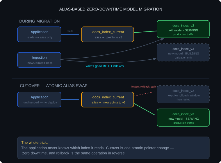
Figure 2-1: Alias-Based Zero-Downtime Model Migration During migration, the application reads through the alias pointing at the old index while new documents are written to both indexes. Cutover is a single atomic alias swap - no application deploy, no downtime, and rollback is the same operation in reverse.
The alias swap is the whole trick - it converts a risky infrastructure migration into a single atomic pointer change with a built-in undo. Weaviate and Qdrant support collection aliases natively. On databases without native aliases, such as Pinecone, the same pattern is implemented one layer up - the application or gateway holds the pointer to the current index name and swaps it atomically in configuration. The cost of this pattern is temporary dual-index storage - you carry two full indexes for the duration of the migration.
Embedding versioning as a first-class concern
When retrieval quality degrades and you need to investigate, the first questions are always the same: which model embedded this document? When? Has the document changed since? If your index cannot answer these questions, every investigation starts blind.
Every vector in your index should carry provenance metadata:
{
  "document_id": "doc_abc123",
  "chunk_id": "chunk_7",
  "embedding_model": "text-embedding-3-large",
  "embedding_model_version": "2024-01-01",
  "embedding_dimension": 1536,
  "embedded_at": "2026-03-15T08:23:41Z",
  "document_hash": "sha256:a3f2..."
}
Two fields do most of the work. embedding_model_version lets you answer "which vectors were produced by the deprecated model?" as a metadata filter rather than a forensic exercise - essential during migrations and after any model update. document_hash - a content hash of the source document at embedding time - turns staleness detection into a cheap comparison: if the current document hash differs from the stored hash, the vector is stale. Without it, detecting staleness means re-reading and comparing every source document against the index - a full corpus scan every time you want to know what needs re-embedding.
This metadata costs almost nothing to store and pays for itself the first time you run a migration or investigate a quality regression. Add it from day one; retrofitting provenance onto an existing index of millions of vectors is exactly the forensic exercise the metadata exists to prevent.
Retrieval evaluation in production
Everything in this chapter so far happens before or during deployment: benchmarking candidates, selecting a model, adapting it, migrating safely. This final section is about what happens after - because retrieval quality is not a property you establish once. It is a property you hold onto, against a corpus that keeps changing and a query distribution that keeps drifting.
Offline evaluation tells you how the model performs on a fixed set of queries at a fixed point in time. It cannot tell you that your users started asking about a product line that launched last month, or that a bulk document import last week polluted the index with near-duplicates, or that retrieval quality has been sliding two percent a week for a month. For that, you need signals from production itself.
Detecting retrieval drift without ground truth
The core constraint of production retrieval evaluation: you do not have labels. Ground truth - the canonical set of relevant documents per query - is expensive to build once and impractical to maintain continuously against live traffic. Production evaluation has to work from signals the system already produces.
Think of it the way a doctor monitors a patient between checkups. The annual physical (your offline eval) is thorough but infrequent. Between physicals, you watch vital signs - heart rate, blood pressure, temperature. None of them diagnoses a specific disease, but a sustained shift in any of them tells you something is wrong and it is time to run real diagnostics. Production retrieval monitoring works the same way: cheap, continuous vital signs that trigger the expensive, precise offline evaluation when they move.
Three vital signs cover most retrieval failure modes:
Retrieval score distribution. Every retrieval returns similarity scores. Track their distribution over time - the median, and especially the tail. A downward shift means documents are being retrieved at lower confidence: either the queries have drifted away from what the embedding model handles well, or the index content has changed underneath it. A narrowing gap between the top-1 and top-5 scores is a subtler version of the same signal - the model is finding it harder to discriminate the best result from the runners-up, which is exactly the dense-cluster ordering problem from Section 1 getting worse in production.
Coverage. Track the rate of queries that retrieve no document above your confidence threshold. Each one is a query your index cannot answer confidently. A rising low-confidence rate is the clearest early warning of query distribution shift - users asking about things the corpus does not cover, or covers with documents the model cannot connect to their phrasing. This signal often moves weeks before users complain, because users who get poor answers usually rephrase or give up rather than file feedback.
Faithfulness as a retrieval proxy. In a RAG system, faithfulness measures how well the generated answer is grounded in the retrieved context. It is primarily a generation metric - but it doubles as a retrieval signal, because a model given weak context has to fill the gaps from parametric memory, and faithfulness drops. The diagnostic rule: a faithfulness regression with no model or prompt change is usually a retrieval regression. Faithfulness measurement itself - how it is computed, at what sampling rate, and at what cost - is covered in Chapter 8 - RAG Evaluation; here it serves as a health signal, not an end metric.
# Retrieval vital signs - computed per time window (e.g., hourly),
# alerted on sustained shifts against a trailing baseline
signals = {
    # Score distribution - alert on downward drift
    "p50_similarity_score": scores.percentile(50),
    "p10_similarity_score": scores.percentile(10),   # tail degrades first

    # Coverage - alert on increase
    "low_confidence_rate": (top1_scores < confidence_threshold).mean(),

    # Discrimination - alert on narrowing
    "top1_top5_score_gap": (top1_scores - top5_scores).mean(),

    # Faithfulness proxy - alert on decrease with no model/prompt change
    "avg_faithfulness_score": faithfulness_scores.mean(),
}
Alert on sustained shifts against a trailing baseline - not on fixed thresholds. Score distributions differ by corpus, model, and query mix; what is a healthy P50 for one system is a degraded one for another. The signal is the trend, not the absolute value.
The feedback loop
These vital signs do not diagnose - they trigger diagnosis. When a signal moves, the response is an offline evaluation run against your eval set. The combination of production signal and offline result tells you where the problem lives:
Production degraded, eval set unchanged → query distribution shift. The model still performs on the distribution you measured - but that is no longer the distribution your users generate. The fix is not a model change: expand the eval set to cover the new query patterns, then re-evaluate whether the current model handles them or domain adaptation is needed.
Eval set degraded too → model or index regression. Something changed in the system itself: a managed embedding API silently updated its model, index staleness crossed the threshold where your eval documents are outdated, or a corpus change introduced documents that confuse retrieval. The eval set localizes it - because the queries are fixed, the change must be in the model or the index.
Both degraded, in different ways → compound issue. Investigate model, index, and corpus independently before touching anything - changing the model to fix what is actually an index staleness problem burns a migration cycle and fixes nothing.
This branching is why the eval set is a permanent asset, not a one-time selection tool. It is the fixed reference point that lets you separate "the world changed" from "the system changed" - the single most common confusion in retrieval quality incidents.
Retrieval quality degradation almost never announces itself as an error. Latency stays flat, error rates stay flat, dashboards stay green - while the system quietly returns lower-quality context and generates confident answers from it. The only defense is instrumenting signals that are sensitive to quality, not just to operational health. If your retrieval monitoring consists of latency and error rate, you are not monitoring retrieval.
The retrieval foundation
The embedding model is the component that determines whether your system can find the right information. Every layer above it - the reranker, the RAG architecture, the agent loop - depends on the retrieval foundation being solid. A well-chosen, properly evaluated, domain-adapted embedding model with production monitoring in place is that foundation. This chapter has been a single argument made several ways: retrieval quality is not something you buy with a model choice - it is something you measure on your own data, select for under your own constraints, adapt toward carefully, and then actively defend in production. The eval set you built runs through all of it: it selects the model, gates the fine-tune, validates the migration, and anchors the drift investigation. Build it once, keep it current, and every retrieval decision afterward has a reference point.
Throughout this chapter, the vector index has been a black box - code samples called vector_search() and moved on. That black box is where the next set of production problems lives: how the index is structured, how it shards across nodes, how it stays fast under concurrent reads and writes, and how quickly a changed document becomes retrievable. That is the subject of the next chapter.
Next: Chapter 3 - Vector Database Architecture, Scaling, and Real-Time Indexing