1 · Workload Characterization: Know What You're Serving

The expensive sizing mistake in production LLM infrastructure is not a wrong GPU choice or a misconfigured parallelism setting. It is skipping workload characterization entirely and jumping straight to hardware selection. Decisions that follow - memory budget, quantization strategy, parallelism degree, batching configuration - is downstream of understanding what you are actually serving.

Before touching a single configuration parameter, key questions must have concrete, data-driven answers.

What model are you serving?
Parameter count, architecture, and the precision you run it at determine your memory floor before a single request arrives.
On architecture: most models today are either dense or Mixture-of-Experts (MoE). A dense model uses every one of its parameters on every forward pass - Llama-3 70B activates all 70 billion weights every time it generates a token. A MoE model like DeepSeek-V3 works differently: it has 671B total parameters but routes each token through only a small subset of specialized "expert" layers - roughly 37B parameters active per forward pass. The headline size is large but the compute and memory pressure per token is much closer to a 37B model than a 671B one. You need to store all the weights but you only pay compute for the active ones.
On precision: neural network weights can be stored at different levels of numerical accuracy - BF16 and FP16 both use 2 bytes per parameter, FP8 uses 1 byte, INT4 uses half a byte. BF16 has become the standard for training because its wider numerical range prevents instability during backpropagation. For inference, precision choice is purely an engineering tradeoff between memory and quality. The same Llama-3 70B model needs 140 GB at BF16/FP16, 70 GB at FP8, and 35 GB at INT4. Lower precision trades a small amount of output quality for large reductions in memory and faster computation. In production inference, FP8 has become the standard starting point on H100 hardware - it halves memory relative to BF16 with negligible quality impact on most tasks.

What does your input length distribution look like - at P50, P90, and P99? Not the average. The distribution. This matters because KV cache memory is allocated per token per active request. A workload whose P99 input is 16K tokens while its P50 is 512 tokens will behave like two completely different systems under load. The P99 case is what causes OOM failures in production.

What does your output length distribution look like? Output length determines how long each request occupies a decode slot, which directly governs throughput. A system serving 50-token outputs can handle dramatically more concurrent requests than one serving 2,000-token outputs on identical hardware.

What is your peak requests per second? Not your average. See section 1.4 on why this distinction is sharper than most teams expect.

What are your latency SLOs, and which metric matters most? TTFT (time to first token), ITL (inter-token latency), and E2E (end-to-end) latency are three different things driven by three different system properties. A system optimized for TTFT may actively degrade ITL, and vice versa. Conflating them leads to configurations that satisfy benchmarks but fail users.

Online streaming or offline batch? These are not different points on the same spectrum - they are fundamentally different optimization targets that call for different architectures entirely.

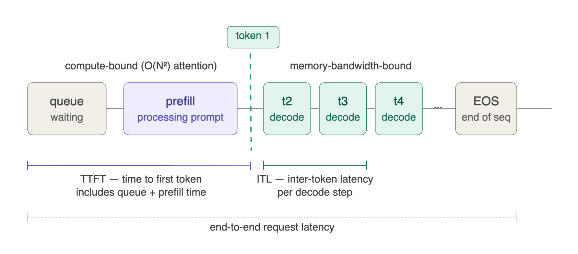
Figure 1.1 - Request lifecycle: TTFT, ITL, and end-to-end latency

A single request passes through three distinct phases. It first waits in queue - this time is often invisible in benchmarks but fully visible to users. Prefill then processes the entire prompt in one compute-bound pass (O(N²) attention), producing the first token; the time from request arrival to this first token is TTFT - time to first token. Each subsequent token is generated one at a time in the decode phase, which is memory-bandwidth-bound rather than compute-bound because the full model weights must be loaded from HBM on every step; the time between consecutive tokens is ITL - inter-token latency. End-to-end latency spans the entire journey from queue entry to the final EOS token. TTFT, ITL, and E2E are three distinct metrics driven by three different system properties - optimizing one can actively degrade another.

1.1 Why P99 Input Length Matters More Than P50

P50 input length is useful for capacity planning at steady state. It is useless for preventing production failures.

Consider a serving system sized for a P50 input of 512 tokens. Under normal load it runs comfortably. Then a burst of P99 requests arrives - each with 32K tokens of context, perhaps from a RAG pipeline retrieving a full document set. Each of those requests allocates 32K × KV-cache-bytes-per-token of GPU memory. If 20 such requests land simultaneously on an instance sized for typical traffic, KV cache is exhausted, new requests are rejected or preempted, and the failure propagates across the batch. The system did not fail because the hardware was wrong. It failed because the sizing assumption was wrong.

The correct approach is to size KV cache headroom for P95 or P99 input length at your target peak concurrency. The median tells you what your system handles most of the time. The tail tells you what breaks it. In production LLM deployments, OOM failures almost always originate at the tail - a workload characteristic that is invisible if you only measure averages. Every sizing decision in this guide is built around that principle: design for the distribution, not the mean.

1.2 Four Workload Archetypes: Each With a Different Hardware Bottleneck

Not all LLM workloads stress the system the same way. There are four distinct archetypes, each with a different dominant bottleneck and a different sizing profile.

Chat and conversational AI - short inputs, short outputs, highly latency-sensitive. TTFT dominates the user experience because humans perceive the pause before the first word. ITL is largely invisible because modern inference engines generate tokens faster than humans read. The hardware bottleneck is prefill throughput at low concurrency, and the key metric is TTFT under load.

RAG pipelines - long inputs (retrieved documents plus query, often filling most of the context window), short to medium outputs. The dominant cost is prefill: processing thousands of input tokens to produce a few hundred output tokens. This is compute-intensive and benefits most from high TFLOPS and quantization that reduces weight movement during prefill. KV cache pressure is high per request but duration is short.

Code generation and long-form reasoning - short to medium inputs, long outputs. The dominant cost is decode: generating hundreds or thousands of tokens autoregressively. This is memory-bandwidth-bound - the system spends most of its time moving model weights from high-bandwidth-memory (HBM) to compute units for each decode step. The key metric is ITL and sustainable decode throughput at high concurrency. This archetype benefits most from high HBM bandwidth GPUs and large batch sizes that get more work done per weight-loading trip.

Agentic and multi-step workflows - the archetype that breaks every simple sizing model. A single user action triggers a chain of sequential LLM calls: planning, tool invocation, result interpretation, re-planning. Context accumulates across turns. Total token consumption per user session is an order of magnitude higher than a single-turn interaction. The challenge here is not peak RPS in the traditional sense - it is sustained GPU occupancy across a session with variable-length, dependent calls. Sizing for agentic workloads requires modeling the entire session token budget, not just individual request characteristics.

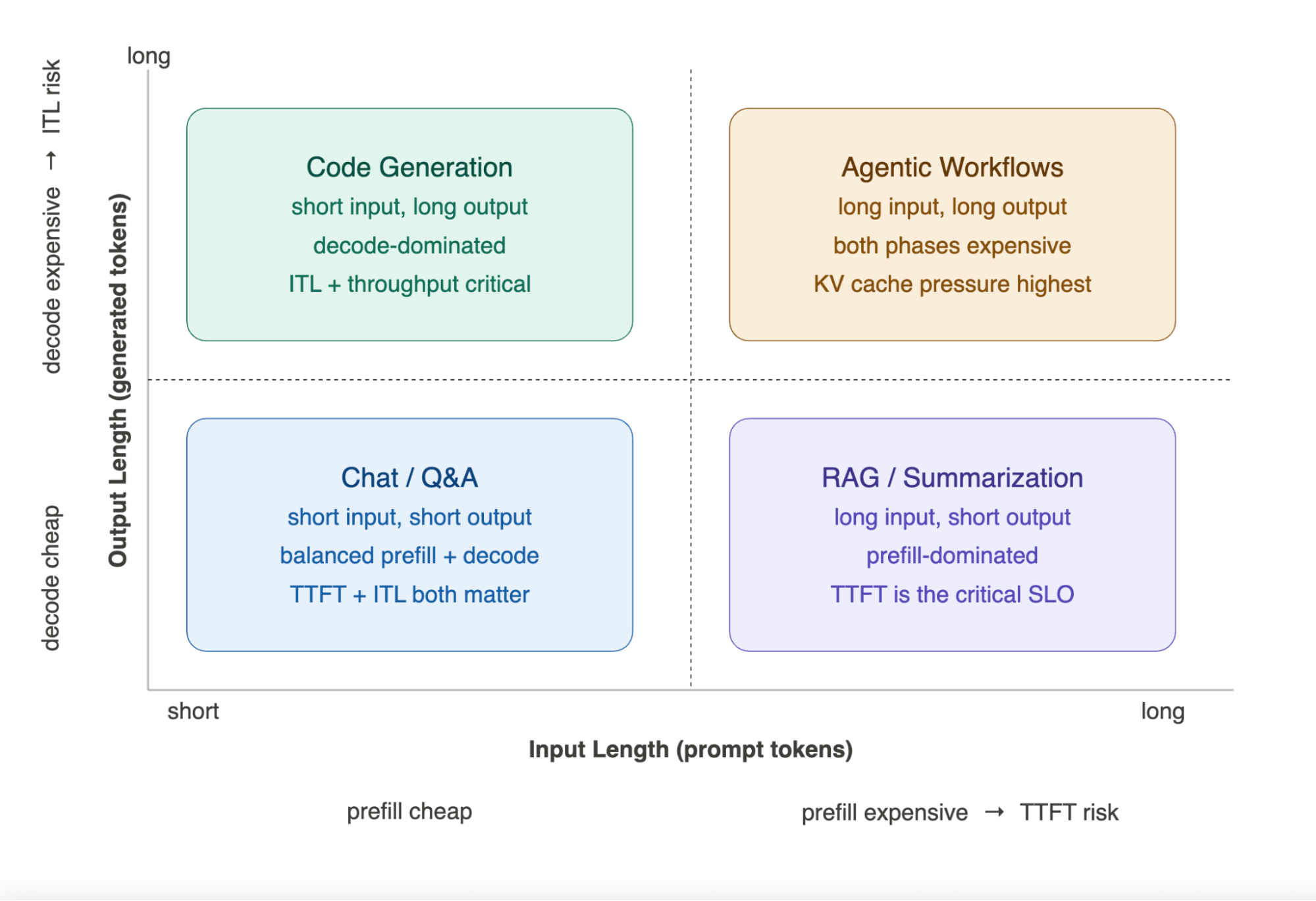
Figure 1.2 - Four workload archetypes: input/output length determines your bottleneck

Position on this grid tells you which hardware resource will constrain you first. Moving right increases prefill cost - longer prompts mean more compute and higher TTFT risk. Moving up increases decode cost - longer outputs mean more HBM bandwidth pressure and ITL risk. Chat/Q&A sits at the origin: balanced and forgiving, both phases cheap. RAG/Summarization moves right: prefill-dominated, TTFT is the SLO that breaks first. Code Generation moves up: decode-dominated, ITL and sustained throughput are what matter. Agentic Workflows occupy the top-right corner: both phases expensive, KV cache pressure highest, and the standard per-request sizing model breaks down entirely.

1.3 Sizing for Peak, Not Average: Request Arrival Patterns

Production traffic is bursty. The Poisson distribution is a reasonable approximation for arrival patterns in many systems, but it has a key property that sizing teams frequently ignore: the gap between average arrival rate and peak arrival rate is largest at low average rates.

A representative enterprise deployment illustrates how badly this plays out in practice. At an average of 65 requests per second, the P95 peak is 160 RPS - roughly 2.5× the mean, and P99 reaches 180 RPS. The overnight trough pulls the daily average down significantly while the business hours peaks drive the actual capacity requirement. Sizing for the average means your fleet is undersized for approximately 8 hours every working day.

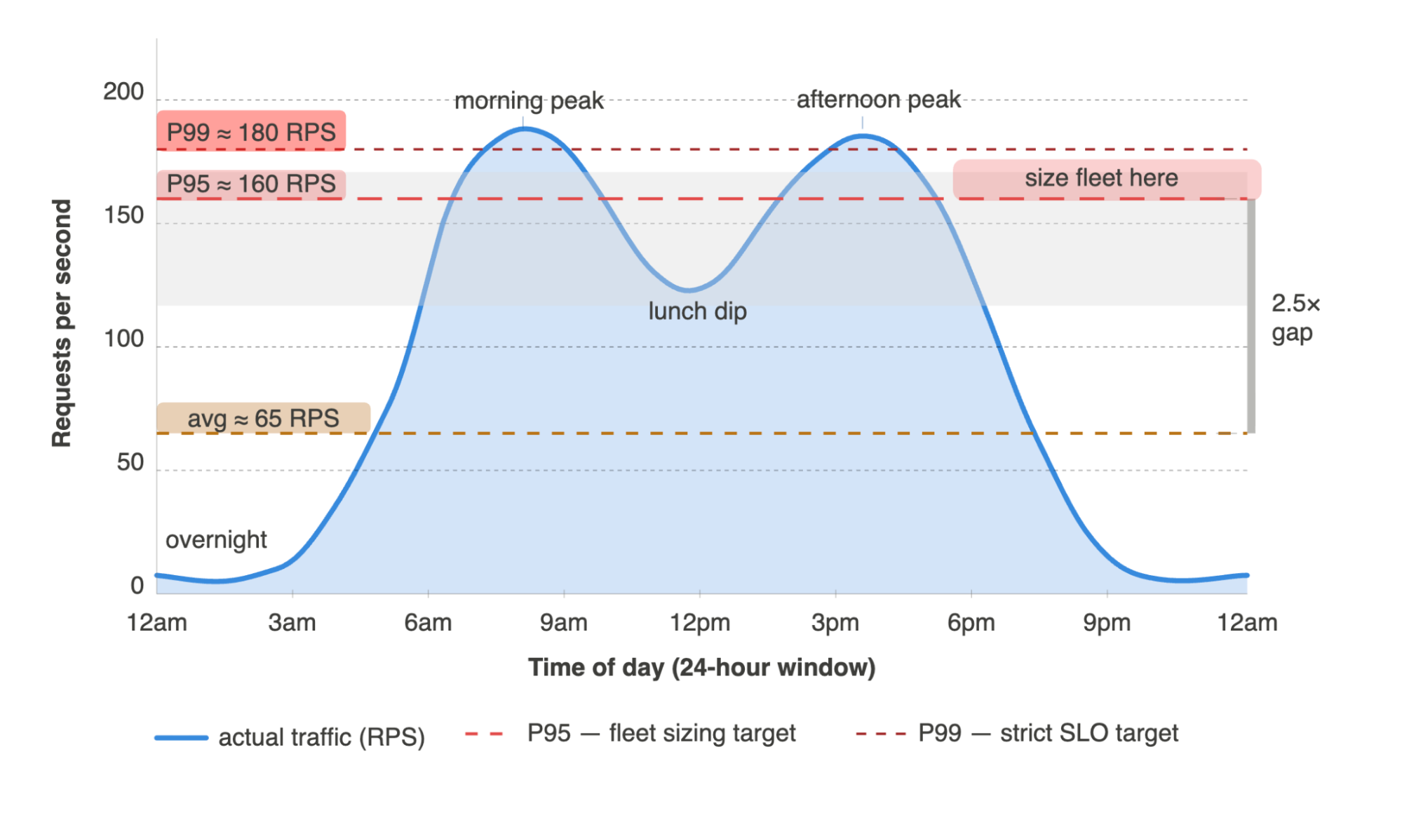
Figure 1.3 - Real enterprise traffic over 24 hours

The gap between average RPS (orange) and P95 RPS (red) is the zone where sizing for average guarantees SLO violations. Both peaks - morning and afternoon - exceed P95 while the overnight trough pulls the average down significantly.

The practical implication: gather actual traffic data, compute the P95 or P99 peak, and size GPU capacity to sustain that peak without SLO degradation. Every downstream calculation in this guide - memory budget, parallelism degree, batch size - assumes P95 as the input, not the average. Sizing for average is not a conservative choice; it is a scheduled outage.

1.4 Online Streaming vs. Offline Batch: Two Optimization Targets

Online streaming and offline batch are not two points on the same dial - they are different optimization problems that require different architectures, different operating points, and different success metrics.

In online streaming mode - where responses stream token by token to a waiting user - generation typically happens faster than human reading speed. Fast readers consume roughly one token every 90ms. Production inference engines generate a token every 15-25ms per request under moderate load. This means ITL is largely invisible to users in streaming mode: the bottleneck on user experience is TTFT, the delay before the first token appears. Systems optimized for online streaming should minimize TTFT, accept some throughput sacrifice to do so, and favor lower concurrency operating points with more aggressive prefill prioritization.

In offline batch mode - document processing, dataset annotation, bulk summarization - no user is waiting. TTFT is irrelevant. The optimization target is pure throughput: maximize tokens generated per GPU-hour, minimize cost per million tokens. Systems optimized for offline batch should operate at maximum sustainable concurrency, use the largest batch sizes that fit in memory, and accept higher latency per request in exchange for higher aggregate throughput.

The failure mode in production is running both workload types on a shared fleet - batch jobs saturate concurrency, TTFT spikes, and latency SLOs degrade while the GPU sits at high utilization doing the wrong work. Offline batch should either fill idle capacity during off-peak hours on latency-optimized fleets, or route to a dedicated throughput fleet entirely.

1.5 Model Routing and Cascading: When One Model Is Wrong

Every sizing calculation in this guide assumes a single model handling all requests - and for many deployments, that assumption holds. Before accepting it for yours, ask one question: do all your requests actually need the same model?

In most production workloads, request complexity is highly skewed. A customer service chatbot handles thousands of "what are your opening hours?" queries for every one complex multi-step reasoning request. A coding assistant handles hundreds of simple autocomplete requests for every architectural design question. If you size a fleet of 70B-parameter GPUs to handle all of these uniformly, you are spending frontier model compute on requests that a 7B model could handle equally well - at roughly 10× lower cost per token.

The fix is a routing layer in front of your fleet that classifies each incoming request by complexity and directs it to the appropriate model tier. This pattern goes by two names that are related but not interchangeable.
Model routing makes the tier decision upfront - the router classifies the request, picks a tier, and sends it there directly.
Model cascading attempts the small model first and escalates to the large model only when the response falls below a quality threshold.

Routing is lower latency because the decision happens once before inference begins. Cascading is more adaptive because it uses actual output quality as the signal, but it pays for that adaptability with a second inference call on every escalated request - which can be 20-40% of traffic depending on your quality threshold. Most production deployments use routing rather than cascading for latency-sensitive workloads. Cascading is better suited to offline batch pipelines where the escalation cost is acceptable and output quality is the primary constraint.

How it works in practice:

Step 1 - Define complexity tiers. Most deployments need only two: a small fast model (7B-13B, heavily quantized, commodity GPUs) for straightforward requests, and a large capable model (70B+, H100s) for complex ones. Some add a third middle tier for moderate complexity.

Step 2 - Build or use a router. The router is a lightweight classifier - either a small fine-tuned model, a rules-based system (input length thresholds, keyword matching), or a learned routing model like RouteLLM - that assigns each request to a tier before it enters the serving stack. The router's latency budget is typically 5-20ms; anything more starts eating into TTFT.

Step 3 - Size each tier independently. This is the critical implication for this guide. Once you introduce routing, you are no longer sizing one fleet - you are sizing two (or more) independent fleets, each with its own memory floor, benchmark curve, SLO-constrained operating point, and GPU count. The sizing algorithm in Section 9 runs separately for each tier.

Cascading follows the same tier structure but reverses the decision logic. Instead of classifying upfront, every request enters the small model tier first. A quality evaluator - typically a lightweight scorer or a confidence threshold on the output - decides whether the response is acceptable. If not, the request escalates to the large model tier and inference runs again from scratch. The sizing implication is different from routing: your small model tier must be sized to handle 100% of peak RPS since every request passes through it, while the large model tier is sized only for the escalation fraction. Cascading is rarely worth the complexity for online workloads but may become attractive for offline batch pipelines where output quality is the primary constraint and the escalation latency penalty is irrelevant.

The TCO impact is substantial. If 70% of traffic routes to a 7B tier running on commodity GPUs and 30% routes to 70B on H100s, your blended cost per token is roughly 0.7×(small cost) \+ 0.3×(large cost) - a significant reduction versus uniform large-model serving. RouteLLM's benchmarks report 40-85% cost reduction in practice depending on quality threshold, which is consistent with this math.

What routing does not fix. Routing adds a new failure mode: misclassification. A complex request routed to the small model produces a poor response; a simple request routed to the large model wastes compute. The router's quality threshold is a dial between cost savings and quality risk - set it too aggressively and you degrade user experience; set it too conservatively and you capture little of the potential savings. Always measure small-model response quality on your specific workload before committing to a routing threshold.

Routing also adds operational complexity - two or more fleets to deploy, monitor, scale, and maintain instead of one. For small deployments this overhead is not worth it. The crossover point is roughly when your large-model fleet would otherwise exceed 8-10 GPUs and your traffic has a measurable skew toward simpler requests.

When to consider routing:

Signal	Recommendation
Traffic is highly homogeneous in complexity	Skip routing - overhead not justified
Clear bimodal complexity distribution (many simple, few complex)	Strong routing candidate
Large model fleet exceeds 8 GPUs	TCO savings likely justify routing complexity
Response quality on small model is measurable and acceptable	Proceed with routing
Latency budget is extremely tight (< 200ms TTFT)	Add router latency to your TTFT budget model before committing; rule out routing if the router alone consumes > 10% of budget.