2 · GPU Memory Sizing: The Hard Constraint
GPU VRAM is not a soft limit you can negotiate around with clever configuration. It is a binary constraint. The system either fits or it does not start. No batching strategy, no parallelism trick, no serving framework feature helps you if the total memory footprint exceeds available VRAM. This makes memory sizing the first engineering calculation, not the last.
When an LLM inference engine starts up, it must allocate four distinct categories of GPU memory before it can serve a single request. These four categories have completely different characteristics - some are fixed at load time, some grow dynamically with traffic, some are model-determined, some are workload-determined - and conflating them is the root cause of most production memory miscalculations.
1. Model weights are the parameters loaded from disk. This is the number everyone calculates. It is fixed the moment the model loads and does not change regardless of traffic. It is also the easiest component to reason about because it depends only on parameter count and numerical precision.
2. KV cache is the stored key and value tensors from the attention mechanism, maintained for every token in every active request. Unlike weights, KV cache is not a property of the model - it does not appear on model cards and cannot be measured offline. It grows dynamically at runtime as a function of sequence length, concurrency, and the number of attention layers. At high concurrency with long context, KV cache routinely exceeds model weight memory by a significant margin. This is the component that will exhaust your VRAM budget before anything else does.
3. Activations are the intermediate tensors computed during the forward pass - the layer inputs, outputs, and attention matrices that exist transiently as each token is processed. They are not stored across requests like KV cache; they exist only during the computation of a single forward pass. However at high batch sizes they accumulate across all layers simultaneously, and their memory footprint scales with batch size, sequence length, and model width. At large batch sizes they become non-trivial - typically 15-30 GB for a 70B model at production concurrency - and ignoring them produces a memory budget that is systematically optimistic.
4. Framework overhead is everything the serving runtime consumes that has nothing to do with the model or the requests. This includes the CUDA runtime itself, the driver context, internal memory pools and allocators maintained by the serving framework - vLLM, TensorRT-LLM, Triton - plus pre-allocated buffers for async scheduling, and the memory fragmentation that accumulates over time in long-running processes. This component is opaque, vendor-specific, and almost never documented. In practice it runs 10-20 GB for mature frameworks on H100s and should be treated as a fixed tax on every deployment regardless of model size.
These four components sum to your total VRAM requirement:
Total VRAM = Model Weights + KV Cache + Activations + Framework Overhead
The formula is simple. The difficulty is that three of the four terms are functions of runtime variables - concurrency, sequence length, batch size - not static model properties. You cannot calculate this from a model card. You must calculate it from your workload characterization.
To make this concrete, consider Llama-3 70B - one of the most commonly deployed frontier-class models - at 50 concurrent requests with 8K context. The numbers are representative of what a real production sizing exercise produces. Here is what the four components actually produce:
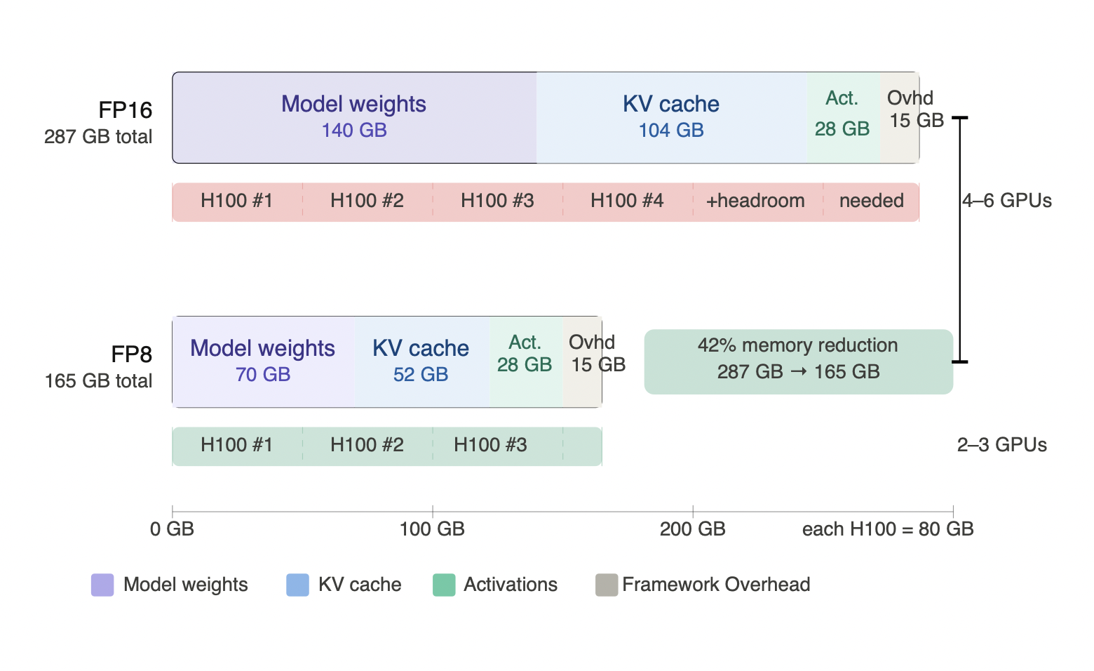
Figure 2.1 - GPU memory breakdown: FP16 vs FP8 for Llama-3 70B (50 concurrent requests, 8K context)
Quantization from FP16 to FP8 halves both model weights and KV cache, reducing total memory from 287 GB to 165 GB. Activations and framework overhead are unaffected by weight precision. The GPU count drops from 4-6 H100s to 2-3 - the single highest-leverage memory decision available before touching throughput.
The sections that follow examine each component in detail - the formula that governs it, the runtime variables that affect it, and the mistakes teams make when they underestimate it.
2.1 Model Weights: The Floor
This is the one everyone calculates. Model weight memory is determined by parameter count and numerical precision.
Model memory (bytes) = num_parameters × bytes_per_dtype
| Precision | Bytes per parameter |
|---|---|
| FP32 | 4 |
| FP16 / BF16 | 2 |
| INT8 | 1 |
| INT4 | 0.5 |
In practice: Llama-3 8B in FP16 needs 16 GB. Llama-3 70B in FP16 needs 140 GB. Llama-3 70B in INT4 needs 35 GB - the difference between requiring a full DGX node and fitting on a single GPU with room to spare. Quantization's impact on memory is this stark, which is why Section 4 covers it as a first-class sizing lever rather than a post-hoc optimization.
The formula is correct but incomplete. Five properties of model weight memory that production engineers learn the hard way:
The alignment tax is real. GPU memory allocators cannot pack tensors like books on a shelf - each tensor requires padding to align to memory boundaries, and that padding accumulates silently across hundreds of layers. In practice, resident weight memory runs 3-8% above what the formula predicts. On a 140 GB model that is 4-11 GB of memory you never explicitly allocated. On a tight configuration, that invisible overhead is what tips you into an OOM at load time.
Weight memory is a loading event, not just a budget line. Most engineers think about weight memory as a static number - the model either fits or it doesn't. But that memory has to travel from storage to GPU before the first request can be served, and the path matters as much as the size.
| Storage path | Effective bandwidth | 70B FP8 (70 GB) cold start | 70B FP16 (140 GB) cold start |
|---|---|---|---|
| Local NVMe (PCIe Gen4) | ~12.5 GB/s | ~6 seconds | ~11 seconds |
| Network-attached (10 GbE) | ~1.1 GB/s | ~64 seconds | ~2 minutes |
| Object storage (S3/GCS) with container init | ~0.5-1.0 GB/s effective | 2-5 minutes | 4-10 minutes |
The object storage row reflects real Kubernetes conditions - raw transfer bandwidth is only part of the cost. HTTP chunked transfer, metadata operations, framework initialization, and container startup all stack on top, pushing cold start times to 2-10 minutes for 70B-class models. This is orders of magnitude longer than web service cold starts, and it breaks reactive autoscaling entirely: by the time a new instance is ready, the traffic spike has already peaked and your SLO has already been violated.
Scale-from-zero is almost never the right pattern for LLM fleets for this reason. Unlike stateless web services where scale-from-zero is economically attractive, LLM fleets pay a 2-10 minute cold start penalty on every scale-up event from zero - a penalty that makes it operationally untenable for any workload with predictable traffic.
Quantization and local NVMe caching of model artifacts are therefore not just cost and memory optimizations - they are autoscaling responsiveness decisions. A 35 GB FP4 model loads in under 3 seconds from local NVMe. A 140 GB FP16 model pulling from object storage may take 10 minutes. That gap determines whether your fleet can absorb a traffic spike before the SLO is breached. Section 9 covers the production patterns - predictive scaling, minimum warm instance count, and NVMe artifact pre-caching - that manage this constraint operationally.
Precision mismatches create transient spikes. Think of it like moving furniture through a doorway - you need more space during the move than you need once everything is in place. Loading FP16 weights and casting to BF16 at runtime briefly holds both representations in memory simultaneously. The same happens when certain layers are kept in higher precision while the rest serve in INT8. The spike is short-lived but it happens at the worst possible moment - initialization - when you have no requests yet to justify the allocation. A configuration that fits at steady state can OOM before it ever serves a token.
LoRA fundamentally changes the multi-tenant weight equation. Base weights are loaded once and shared across every adapter variant running on that instance. Each LoRA adapter adds only its delta - typically 1-5% of base model size. The practical implication is that serving ten fine-tuned variants of Llama-3 70B costs approximately the same weight memory as serving one. This is one of the most underutilized cost levers in multi-tenant deployments. Subsequent sections cover the full model, but the property originates here.
Serialization format affects load behavior, not resident size. Once loaded, a model in safetensors and the same model in a pickle-based format occupy identical GPU memory. The difference is how they get there. Safetensors supports memory-mapped loading - the OS pages in only what is needed, and the process never holds a full second copy during deserialization. Pickle-based formats require a full deserialization pass that temporarily allocates a second buffer alongside the model being loaded. On a memory-constrained system, that transient second allocation is enough to fail initialization even when the model itself fits.
Overall model-weight memory is the floor. The system cannot initialize below this threshold. Everything that follows is overhead stacked on top of it - and the next component will, in most production workloads, exceed it.
2.2 KV Cache: Where Production Systems Run Out of Memory
This is the component most teams underestimate, often catastrophically. KV cache does not appear in model cards. It is not a static property of the model. It grows dynamically at runtime with every token in every active request - and at high concurrency with long context, it routinely exceeds model weight memory by a significant margin.
The formula:
KV_cache (bytes) = 2 × num_layers × num_KV_heads × head_dim × seq_len × concurrency × bytes_per_element
The factor of 2 is for both the key and value vectors stored per layer. Everything else scales with your workload.
A concrete example grounds the math. Llama-3 70B in FP16 has 80 layers, 8 KV heads, and a head dimension of 128 - working out to approximately 0.26 MB of KV cache per token per request.
At a typical production load of 50 concurrent requests with 8K-token inputs, that is 106 GB of KV cache sitting alongside the 140 GB of model weights on the same system. Already more than 70% of the model's own footprint, just from active requests.
Now extend the context. At 32K tokens the KV cache grows to 416 GB at the same concurrency - three times the model weights. At 128K context, just 4 concurrent requests push KV cache past model weights entirely. The diagram below makes this viscerally clear: short-context workloads stay manageable, but as context length grows the KV cache stops being overhead and becomes the dominant memory consumer in the system.
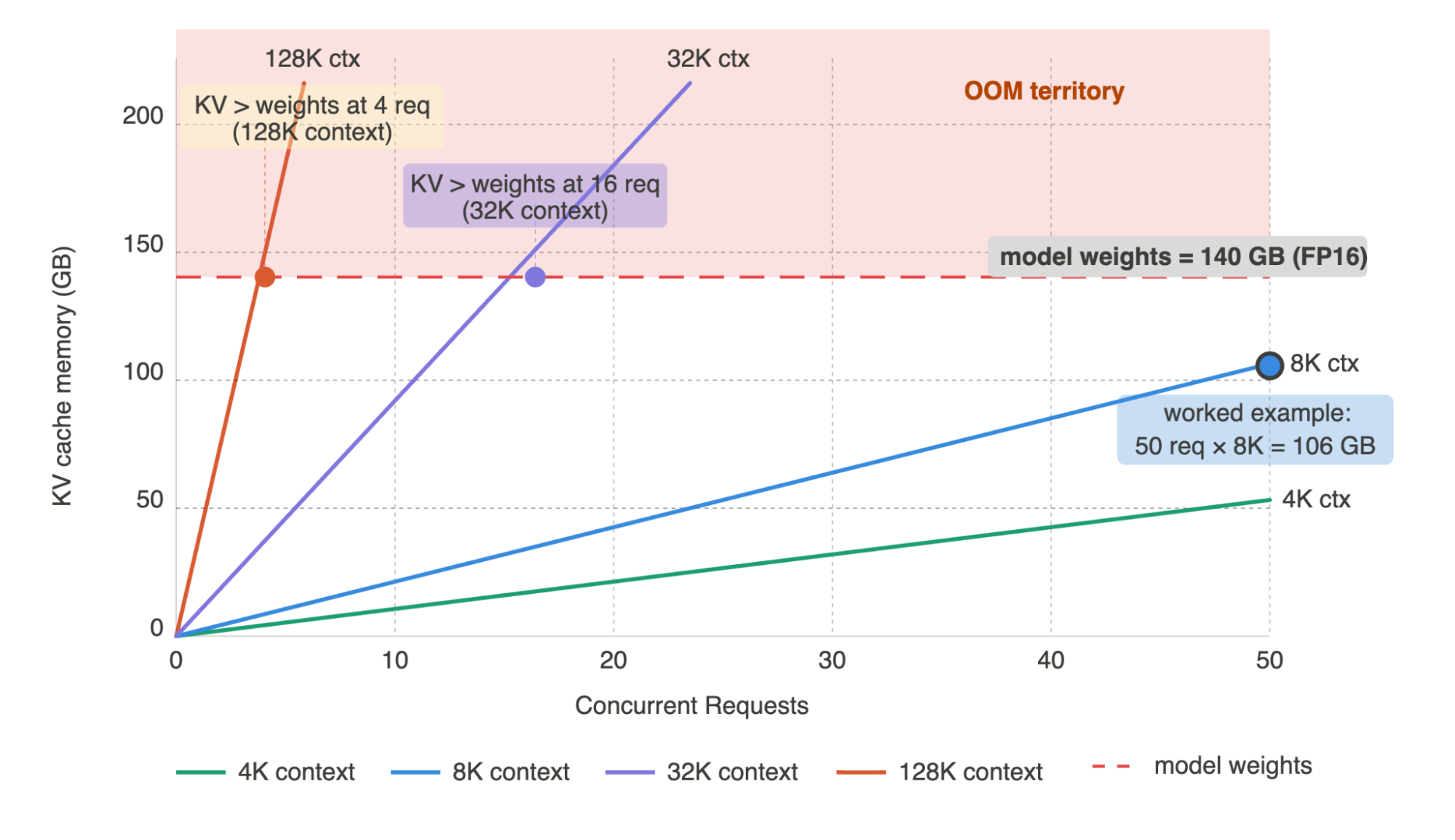
Figure 2.2 - KV cache memory vs concurrency for Llama-3 70B (FP16)
Each line represents a different context length. KV cache grows linearly with concurrency - but the slope scales directly with context length, making long-context workloads disproportionately memory-intensive. At 128K context, model weights are exceeded at just 4 concurrent requests. At 32K context, the crossover happens at 16. Only short-context workloads (4K-8K) stay below model weight memory at typical production concurrency. Size for your P95 context length, not your average.
This is not an edge case. It is the normal operating condition for any RAG pipeline or long-context deployment running at meaningful concurrency. The system sized for the model alone will OOM under realistic load. Every production deployment must calculate both components and sum them before selecting a GPU configuration.
One architectural variable has an outsized effect on KV cache size that is easy to miss if you only read the model card: the ratio of query heads to KV heads. During decode, each token attends to all previous tokens to decide what information to carry forward. Rather than doing this once, transformer models do it multiple times in parallel - each "head" captures a different type of relationship (syntactic, semantic, positional). Each head maintains its own Key and Value vectors, which are what get stored in the KV cache. With 64 heads and a 4K-token context, you are storing 64 sets of K and V vectors per token per layer - which is where KV cache memory comes from.
Multi-Head Attention (MHA) is the standard: every query head has its own dedicated KV head. A model with 64 attention heads stores 64 KV head pairs per token. During decode, every one of those must be loaded from HBM on every step.
Grouped Query Attention (GQA) makes a practical observation: multiple query heads can share the same Key and Value vectors without meaningfully hurting quality - they still ask different questions (each has its own Q vector) but consult the same shared reference material (shared K and V). Think of a committee where every member forms their own opinion independently, but they all read from the same shared briefing document rather than maintaining separate personal copies. GQA reduces KV head count dramatically while preserving model quality.
Llama-3 70B has 64 query heads but only 8 KV heads - an 8× reduction in KV cache size relative to a standard MHA model of the same scale. Modern architectures including Llama-3, Mistral, Qwen, and Gemma all use GQA for exactly this reason - it is one of the primary reasons these models are more memory-efficient during serving than older architectures of comparable parameter count.
When estimating KV cache memory for a model you have not deployed before, always check the KV head count explicitly - not the total attention head count. They are often not the same number, and using the wrong one will cause you to overestimate KV cache memory significantly.
2.3 Activations: The Necessary but Manageable Component
Every forward pass through a transformer layer produces intermediate tensors that must stay resident in memory until the next operation consumes them. These are not stored across requests the way KV cache is - they exist only for the duration of a single forward pass - but at large batch sizes they accumulate across all layers simultaneously and their footprint is non-trivial.
The historical problem was severe. In standard attention, every token must attend to every other token to decide what information to carry forward. With a sequence of N tokens, that produces an N×N attention matrix - one entry for every token-to-token relationship. At 8K tokens that matrix is 64 million entries. At 32K tokens it is over a billion. Memory consumption scaled as O(seq²), meaning doubling context length quadrupled activation memory. Long-context workloads were genuinely dangerous to run at scale under the original formulation.
FlashAttention eliminates the quadratic scaling, but it is worth understanding exactly how. The insight is that you never actually need the full N×N matrix in memory at once - you need the result of multiplying it by the value vectors, which is a much smaller tensor. FlashAttention computes this result incrementally by processing the attention computation in small blocks that fit entirely in the GPU's fast on-chip SRAM, which is orders of magnitude faster to access than HBM but also much smaller. Each block computes its contribution to the final output, accumulates the result, then discards the intermediate attention scores before moving to the next block. The full N×N matrix is never materialized anywhere. Think of it like computing a sum of a million numbers by adding them in groups of a hundred - you never need to write down all million numbers simultaneously, just maintain a running total.
The memory consequence is that activation scaling drops from O(seq²) to approximately O(seq) - linear rather than quadratic. Doubling context length roughly doubles activation memory rather than quadrupling it. This is what makes 32K and 128K context workloads operationally viable on real hardware.
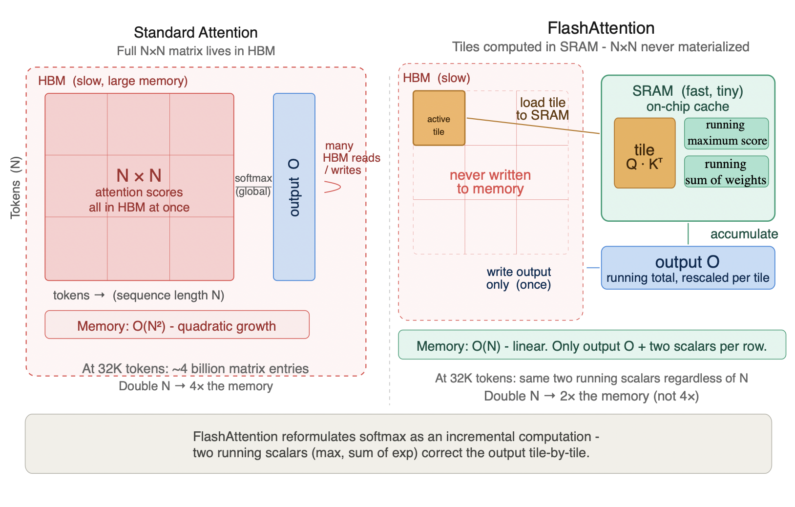
Figure 2.3 - Standard attention vs FlashAttention memory model
Standard attention materializes the full N×N score matrix in HBM before softmax can run - memory grows quadratically with sequence length. At 32K tokens that is roughly 4 billion matrix entries. FlashAttention eliminates this by computing attention in tiles that fit entirely in on-chip SRAM, maintaining only two running scalars per row - a running maximum and a running sum of exponentials - that allow softmax to be computed correctly without ever seeing the full matrix. Memory drops from O(N²) to O(N). The N×N matrix is never written anywhere. This is what makes 32K and 128K context workloads physically viable on current hardware.
FlashAttention is now standard across all major inference frameworks - vLLM, TensorRT-LLM, and Triton all use it by default. You do not need to enable it manually. But understanding what it does matters for sizing because it changes the activation memory model entirely: you are no longer dealing with a component that explodes with context length, you are dealing with one that grows predictably and stays bounded relative to model size.
In practice, budget approximately 20% of model weight memory for activations under FlashAttention. For Llama-3 70B that is roughly 28 GB - significant, but predictable and stable across context lengths in a way that KV cache is not. Unlike KV cache, activations do not creep upward as concurrency or context grows beyond your sizing assumptions. Once you have calculated model weight memory, the activation budget follows directly from it.
This makes activations the most manageable of the four components: not negligible, not ignorable, but calculable from a single number you already know.
2.4 Framework Overhead: The Remainder You Cannot Ignore
Every inference framework - vLLM, SGLang, TensorRT-LLM - is not just a thin wrapper around model execution. It is a runtime system that manages memory pools, request queues, block tables, batching state, and CUDA contexts. All of that infrastructure lives in GPU memory.
Think of it like moving into a new apartment. Before you bring a single piece of furniture, the building has already consumed square footage for the lobby, the stairwell, the electrical room, and the maintenance closet. You never get to use that space for living. Framework overhead works the same way - it is the infrastructure tax paid before the workload begins, and it is non-negotiable.
What drives the number varies by framework. vLLM pre-allocates block tables for PagedAttention proportional to your configured memory pool size. TensorRT-LLM pre-allocates engine execution buffers at build time, sized to your declared maximum batch size and sequence length - build for batch 128 at 32K context and those buffers are reserved regardless of actual traffic. SGLang maintains a radix cache structure for prefix reuse that adds its own allocation on top of the base CUDA runtime.
The practical budget is 5-10% of total VRAM on top of the other three components. On an 80 GB H100 that is 4-8 GB that is structurally unavailable regardless of what the model card says. This is why systems that look viable on paper occasionally fail to initialize - the calculation accounted for weights, KV cache, and activations, but not the framework claiming its share first.
2.5 Multi-LoRA Serving: Memory Implications
For deployments serving a single model variant, the four components above complete the memory budget. Most enterprise deployments do not serve a single variant. A customer service platform might run dozens of domain-specific fine-tunes of the same base model - one for billing, one for technical support, one per language. Fine-tuning a 70B base model for each use case and deploying separate instances is prohibitively expensive. Fine-tuning does not require retraining the full model - it produces a small set of weight adjustments called an adapter that captures only the task-specific changes, typically 50-200 MB versus 140 GB for the full 70B weights. Multi-LoRA serving solves this by sharing the base model weights across all tenants while loading only the lightweight adapter weights per request - a single GPU fleet serves dozens of fine-tuned variants without duplicating the base model.
The memory math is straightforward but frequently miscalculated in production:
Base model memory - unchanged. The full model weights at target precision load once and are shared across all LoRA variants.
LoRA adapter memory - each adapter adds a small memory overhead. A LoRA adapter for a 70B model with rank r=16 typically adds 50-200 MB per adapter depending on which weight matrices are adapted (Q, K, V, FFN, or all).
The rank (r) controls the adapter's expressive capacity. Each weight matrix in the model is a large 2D grid of numbers - LoRA does not modify it directly. Instead it learns two small rectangular matrices that together approximate only the change needed from fine-tuning: one narrow matrix (rank × full dimension) and one flat matrix (full dimension × rank). Multiplied together they reconstruct a full-size update, but constrained to patterns expressible within r independent directions. Think of it like describing a complex piece of music using only r instrument tracks - rank=4 gives you 4 tracks to approximate the full arrangement, rank=64 gives you 64. More tracks means finer detail but larger memory footprint. The base model weights never change - you are only storing and swapping the lightweight adapter matrices.
Most production deployments use r=8 to r=64. Crucially, only the adapters for currently active requests need to reside in GPU memory - inactive adapters can be paged out to CPU memory and loaded on demand.
Peak adapter memory - the binding constraint is not the total number of adapters but the maximum number of distinct adapters simultaneously active in the batch. If your batch of 50 concurrent requests spans 8 distinct LoRA variants, you need memory for 8 adapters simultaneously, not 50.
Total memory = base_model_memory + (max_simultaneous_adapters × adapter_size) + KV_cache + activations
The failure mode teams hit in production. A deployment serving 100 LoRA adapters assumes adapter memory is negligible because each adapter is small. Under bursty traffic, requests for many distinct adapters arrive simultaneously, all 100 adapters get loaded into GPU memory concurrently, and the deployment OOMs - not because of the base model or KV cache, but because of adapter accumulation. The fix is to cap max_simultaneous_adapters in your serving configuration and implement LRU eviction for inactive adapters.
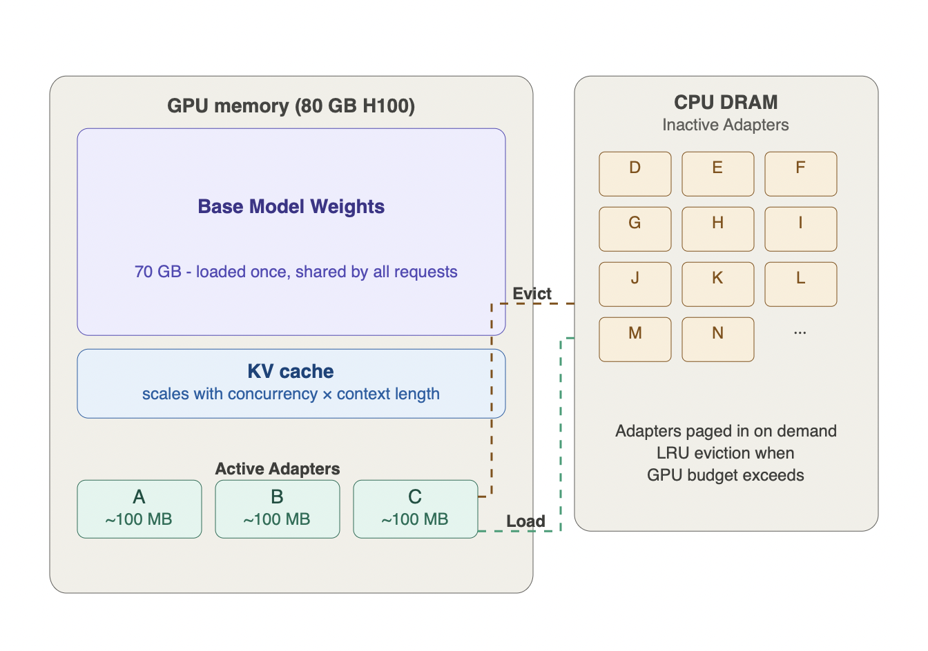
Figure 2.5 - Multi-LoRA serving memory architecture
The base model loads once and is shared across all tenants. Only adapters for currently active requests reside in GPU memory - inactive adapters are paged to CPU DRAM and loaded on demand via LRU eviction. The binding constraint is not the total number of adapters but the maximum number simultaneously active in the batch. The failure mode: bursty traffic causes all adapters to load concurrently, exhausting GPU memory - not from the base model or KV cache, but from adapter accumulation.
Framework support. vLLM supports multi-LoRA serving natively with configurable max_loras (number of adapters in GPU memory simultaneously) and max_lora_rank. SGLang supports multi-LoRA with similar controls. Both implement adapter paging - loading adapters from CPU to GPU on demand and evicting LRU adapters when the GPU memory budget is exhausted.
2.6 Putting It Together: The Minimum GPU Count Formula
Every component in this section was building toward a single calculation. You now have everything you need.
Min GPUs = ceil((model_weights + KV_cache_at_peak_concurrency + activations + overhead + (max_simultaneous_adapters × adapter_size)) / GPU_VRAM)
The KV cache term is the variable that changes everything. It is a function of your workload - context length, concurrency, and model architecture - not a property of the model alone. Two teams running the same model on the same GPU will get completely different minimum GPU counts if their concurrency and context length assumptions differ. This is why workload characterization in Section 1 comes before GPU selection, not after.
Worked example: Llama-3 70B in FP16, 50 concurrent requests at P95 input length of 8K tokens, H100 80 GB.
Model weights come in at 140 GB. KV cache at this concurrency and context length works out to 50 × 8,000 × 0.26 MB ≈ 104 GB. Activations add roughly 28 GB and framework overhead another 15 GB. Total: approximately 287 GB - which requires ceil(287 / 80) = 4 H100s at minimum, with essentially no headroom for anything.
If you are serving 8 simultaneous LoRA adapters at rank=16, add roughly 0.8 GB - negligible at this scale, but meaningful at high rank or large simultaneous adapter counts.
Now apply FP8 quantization. Model weights drop to 70 GB, KV cache drops to 52 GB, total falls to approximately 165 GB, and 2-3 GPUs become viable. That is the leverage quantization provides at the memory sizing stage - before throughput, before latency, before any other optimization. It is a GPU count decision, not a quality tuning decision.
On headroom. The minimum GPU count is not your deployment GPU count. A system running at 95% VRAM utilization is one traffic burst away from an OOM cascade. Add 30-50% headroom beyond the calculated minimum: enough to absorb spikes above P95, keep the system away from the memory cliff edge, and survive framework version updates that quietly increase overhead between deployments. For the FP16 example above, that headroom recommendation moves the practical minimum from 4 GPUs to 6. For the FP8 case it moves from 2-3 to 3-4 - still a meaningful saving over the FP16 baseline.