6 · Batching Strategy: From Static to Continuous to Disaggregated
Parallelism determines how many GPUs serve a model. Batching determines how efficiently those GPUs are used. A perfectly parallelized deployment running at batch=1 wastes most of its hardware - the roofline analysis showed exactly why: decode is memory-bandwidth-bound, and arithmetic intensity scales linearly with batch size. This section covers the scheduling strategies that close the gap between theoretical and realized throughput.
The stakes are concrete. A GPU holding a 70B model has the same VRAM whether it serves 1 concurrent request or 50. The difference in revenue per GPU-hour between those two operating points is entirely a function of batching strategy and scheduling policy - not hardware. Each evolution in batching covered in this section represents a discrete, measurable throughput improvement deployable on your existing fleet.
This section traces that evolution in order. Static batching fails structurally and the reasons are worth understanding precisely. The scheduler is the mechanism that makes everything else possible. Continuous batching is the production baseline that every serious deployment should already be running. Chunked prefill refines it further. Disaggregated prefill-decode is the architectural leap that unlocks the largest gains. Speculative decoding attacks a different bottleneck entirely - it does not change how requests are batched but how individual decode steps are executed, which is why it appears here as a complement to the batching strategies rather than a replacement for them.
6.1 Static Batching: Why It Fails
Static batching is the naive approach: collect N requests, pad all sequences to the length of the longest one, process the batch as a fixed group, return all results, then start the next batch.
The failure has two distinct mechanisms that are worth separating because they require different solutions.
The first is padding waste. All sequences in a static batch must be the same length for the GPU to process them as a single tensor operation. Every sequence shorter than the longest one is padded with dummy tokens to match. The GPU performs real computation on those padding tokens - consuming memory bandwidth and compute cycles - and produces output that is immediately discarded. At high input length variance, a substantial fraction of every batch's compute budget is spent on padding that contributes nothing to useful output.
The second failure is tail latency blocking. LLM output lengths vary dramatically per request - a simple factual question might complete in 20 tokens while a code generation request runs to 800. In a static batch, the GPU cannot start the next batch until every request in the current batch has finished generating its last token. A single long-running request holds the entire batch hostage. Shorter requests that finished 10 seconds ago sit with completed results while the GPU continues generating tokens for the one slow request. During that wait, the GPU is producing output for exactly one request - the utilization equivalent of batch=1 - while the memory footprint of the entire batch is still occupied.
At high output length variance - which is the norm in any production LLM deployment - GPU utilization collapses for this reason. Static batching is not a suboptimal scheduling policy that can be tuned. It is architecturally incapable of handling variable-length autoregressive generation efficiently. The padding and tail latency problems are structural, not implementation deficiencies.
The solution requires a fundamentally different scheduling model - one that treats the active request set as a dynamic, continuously changing collection rather than a fixed group processed start-to-finish. That is what the continuous batching scheduler does. But before getting to continuous batching, it is worth understanding the scheduler itself as a standalone component, because the scheduler is what makes every subsequent optimization in this section possible.
6.2 The Scheduler: A First-Class Component
Before discussing any batching strategy, it is worth being precise about what a scheduler actually controls - because every batching strategy in this section is, at its core, a scheduling policy decision.
The LLM inference scheduler operates at the iteration level. On each forward pass, it decides three things: which requests are included in the current batch, how many tokens from each request are processed in this step, and what priority ordering governs admission when the batch is full. These decisions directly determine TTFT, ITL, queue depth, and GPU utilization - simultaneously and in tension with each other.
The complication that makes LLM scheduling harder than a simple queue is that requests have two distinct phases - a compute-intensive prefill and a memory-bandwidth-bound decode - and the scheduler must balance both simultaneously on the same hardware. A decision that improves TTFT for new arrivals directly degrades ITL for requests already in decode. Every scheduling policy is a choice about whose experience to protect. Understanding the scheduling policy families is the prerequisite for every batching decision that follows.
The four scheduling policy families - and what they cost you
Think of the GPU batch as a shared highway lane. The scheduler decides who gets to enter, in what order, and whether anyone can be overtaken. The choice of policy determines whose experience degrades when the lane gets congested.
FCFS (First-Come-First-Served) is the default in vLLM and most production frameworks - a strict queue in arrival order, regardless of prompt length or latency deadline. Simple to implement, blind to consequences. The problem is the slow truck on the highway: a single 64K-token request ahead of ten short chat requests blocks all of them, inflating their P99 latency. Input length variance in production is heavy-tailed, so this failure mode is not rare - it is the norm under mixed workloads.
Prefill-priority scheduling lets new arrivals cut to the front of the queue, immediately running their prefill step ahead of ongoing decodes. New users get their first token fast - TTFT improves. Every user already mid-response experiences a stutter - their ITL spikes by exactly the duration of the incoming prefill. At high arrival rates with long prompts, this produces continuous jitter that makes streaming feel broken even when average latency is within budget. The tradeoff is mathematically exact: prioritizing prefill reduces TTFT and unavoidably worsens time-between-tokens in a colocated system.
Decode-priority scheduling is the opposite: protect active responses from any interruption. ITL is stable and predictable. New requests queue and wait - TTFT grows linearly with queue depth. TensorRT-LLM and FasterTransformer use this approach, fully completing current batches before admitting new ones. Under high load, new users wait seconds before seeing their first token while the GPU serves everyone already in flight.
SLO-aware priority scheduling is the production answer to all three failure modes. Instead of ordering by arrival time or phase type, it tracks each request's remaining latency budget. A request close to violating its TTFT deadline moves to the front. A request with 800ms of budget remaining yields to one with 50ms left - regardless of who arrived first. This is what makes interactive chat, batch summarization, and RAG pipelines coexist on a shared fleet without one class consistently cannibalizing another's SLO.
SLO-aware scheduling requires estimating each request's remaining generation time - which is non-trivial since output length is not known at admission in autoregressive generation. Production implementations use either output length predictors trained on historical workload distributions, or conservative deadline tracking based on worst-case output length assumptions. The prediction accuracy directly affects scheduling quality - a poor output length estimator degrades SLO-aware scheduling toward FCFS behavior in practice.
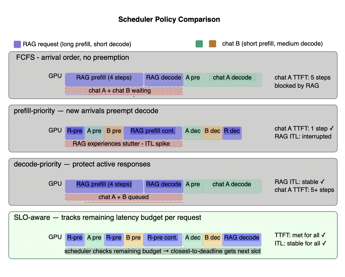
Figure 6.2 - The four scheduler policies: same three requests, four different outcomes
Three requests arrive in sequence: a RAG query with a long prefill, and two short chat requests. Each row shows how the GPU is allocated under a different scheduling policy. FCFS (top) processes requests in strict arrival order - the long RAG prefill blocks both chat requests, inflating their TTFT by 5 steps with no awareness that they had tighter latency budgets. Prefill-priority (second) admits chat A and B immediately, giving both fast TTFT - but RAG's decode is interrupted each time a new prefill arrives, causing ITL spikes that make streaming feel broken. Decode-priority (third) protects active responses from any interruption - RAG's decode is smooth, but chat A and B wait 5+ steps before seeing their first token, with TTFT growing linearly with queue depth. SLO-aware (bottom) tracks each request's remaining latency budget and routes the closest-to-deadline request first - all three requests meet their TTFT and ITL targets simultaneously. The summary table shows why FCFS and single-phase policies consistently fail mixed production workloads.
Why the scheduler matters before choosing a batching strategy. The scheduler determines which requests are in the batch when a prefill arrives, how aggressively prefill is chunked, and how decode requests are prioritized in disaggregated serving. A sophisticated batching architecture running on FCFS will consistently underperform a simpler architecture with an SLO-aware scheduler - the scheduling policy sets the ceiling on what any batching optimization can achieve.
6.3 Continuous Batching: The Baseline
The scheduler policies govern how requests compete for the batch. Continuous batching changes the more fundamental question underneath that competition: when does the batch itself turn over? Before continuous batching existed, the serving system made one scheduling decision per batch: assemble N requests, run them all to completion, then accept new ones. The GPU idled whenever any request finished early - and with variable output lengths, that happened on nearly every batch.
The fix - first formalized in the Orca research paper (OSDI 2022) and now implemented in every serious framework under different names - is iteration-level scheduling. After every single forward pass, completed requests are evicted and new ones are admitted immediately. The GPU stays continuously occupied rather than waiting for the slowest request in each group to finish. vLLM calls it continuous batching. TensorRT-LLM calls it in-flight batching. SGLang and TGI use the same mechanism under their own implementations. The concept is identical across all of them.
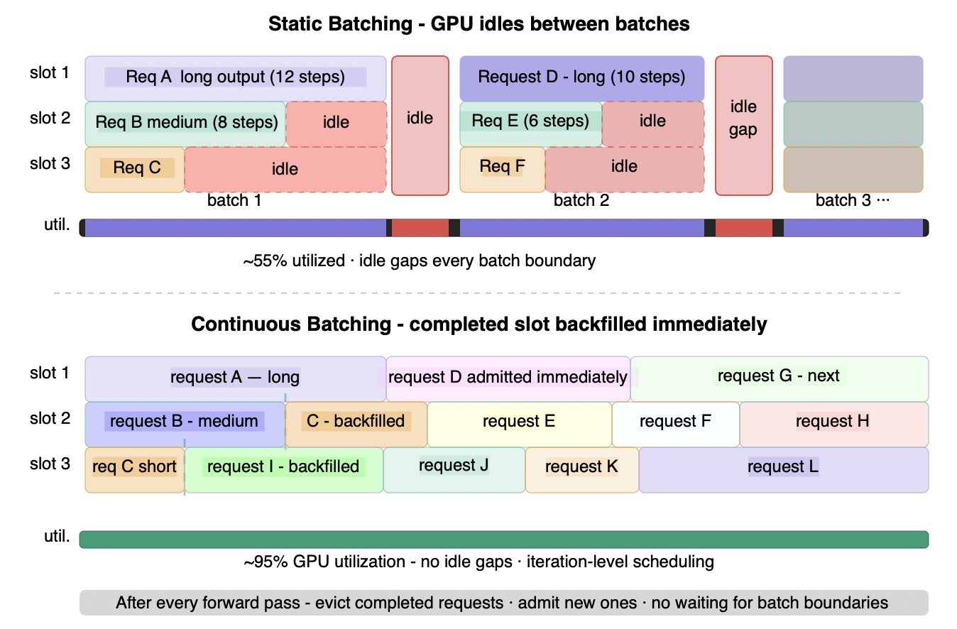
Figure 6.3 - Static batching vs continuous batching: GPU slot utilization
Static batching (top) runs each batch to full completion before admitting new requests. Shorter requests finish early and their slots sit idle - waiting for the slowest request. The inter-batch gap makes it worse: the GPU goes fully dark at every batch boundary. Continuous batching (bottom) makes one scheduling decision per forward pass. The moment any slot completes, a new request fills it - no batch boundaries, no idle gaps, no waiting. The utilization improvement is structural, not incremental: from ~55% to ~95% on the same hardware, serving the same requests.
This is table stakes. If your serving stack does not support it, nothing else in this section will help. But enabling continuous batching is not the end of the story - it introduces three production challenges that must be managed explicitly.
KV cache pressure is the primary operational risk. Continuous batching maximizes GPU slot utilization, which simultaneously maximizes concurrent KV cache consumption. At high throughput, the KV cache fills completely and new requests cannot be admitted even though the GPU has compute headroom. The system hits a memory wall before a compute wall. This is the most common failure mode for teams that enable continuous batching without tuning their KV cache budget. It is also why continuous batching and PagedAttention are inseparable in production - PagedAttention's dynamic memory allocation is what prevents KV cache fragmentation from artificially capping concurrency below what the raw memory budget would allow.
Preemption is the safety valve - and it has a cost. When the KV cache fills completely and a high-priority request must be admitted, the scheduler must evict an active request's KV cache from GPU memory. This happens either by swapping KV tensors to CPU DRAM - adding memory bandwidth overhead - or by discarding them entirely and recomputing from scratch when the request is resumed - adding compute overhead proportional to the evicted context length. Under sustained high load with aggressive admission, preemption frequency rises and P99 latency degrades significantly even when average latency looks healthy. Preemption events are a critical production metric to monitor - a sudden spike in preemption rate is an early warning that your KV cache budget is too small for your current traffic pattern.
Admission control determines P99 behavior under load. Continuous batching without admission control accepts every request immediately and preempts existing ones to accommodate them when necessary. Continuous batching with admission control queues new requests when the KV cache budget is exhausted rather than preempting. This is a configuration choice that most teams leave at framework defaults without understanding the tradeoff: queuing protects P99 latency for active requests at the cost of higher TTFT for new arrivals; preemption protects TTFT at the cost of latency spikes for requests that get evicted. The right choice depends on which SLO your workload weights more heavily - and it should be an explicit decision, not a default.
The utilization gain scales with output length variance. The ~55% to ~95% improvement in the figure above reflects a high output length variance workload - the typical production scenario for mixed chat, RAG, and code generation traffic. For workloads with low variance - batch document processing where every document produces roughly the same output length - continuous batching provides smaller gains because the tail latency blocking problem is smaller to begin with. If you enable continuous batching and see modest throughput improvement, measure your output length distribution before concluding the implementation is wrong. The workload profile may simply not benefit as strongly.
6.4 Chunked Prefill: Interleaving Without Full Separation
Continuous batching keeps the GPU continuously occupied. What it does not solve is the interference between a new request's prefill and active decode requests competing for the same forward pass. A long prefill still stalls every decode in the batch for its full duration - 300-500ms on an H100 for a 16K-token prompt on a 70B model. Chunked prefill is the targeted fix for that specific problem, without requiring separate hardware.
The idea from SARATHI is straightforward: instead of processing the full prompt in one blocking step, split it into fixed-size chunks - say 256 tokens - and process one chunk per iteration alongside ongoing decode requests. No single iteration is monopolized by a long prompt. Decode requests continue generating tokens between every chunk.
This works because of the roofline insight from earlier sections applied directly. A prefill chunk is compute-bound - it saturates CUDA cores. Decode requests in the same batch are memory-bandwidth-bound - they saturate HBM. They consume different hardware resources simultaneously, which means batching them together in the same forward pass approaches both ceilings at once rather than alternating between them. GPU utilization improves as a direct consequence.
Think of it like a highway where a single articulated truck - a full 16K prefill - used to block all traffic for 300-500ms every time it entered the road. Chunked prefill breaks that truck into a convoy of smaller vehicles. Each segment takes its turn in the shared flow of traffic, and the motorcycles (decode steps) keep moving between each segment. The road is still shared - nobody gets their own lane. But no single vehicle monopolizes it long enough to cause a visible stall. That separation into dedicated lanes is what disaggregation in the next section actually does.
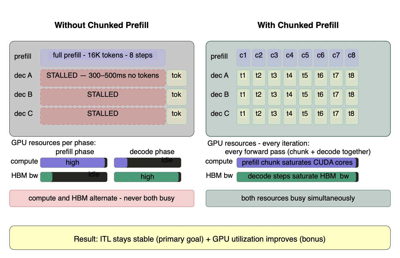
Figure 6.4 - Chunked prefill: ITL stability and GPU utilization
Without chunked prefill (left), the GPU alternates between two extremes - compute saturated and HBM idle during full prefill, then HBM saturated and compute idle during decode. Every active decode request stalls completely for 300-500ms while the long prefill runs. With chunked prefill (right), each forward pass contains both a 256-token prefill chunk and decode steps from all active requests. The prefill chunk saturates CUDA cores. The decode steps saturate HBM bandwidth. They use different hardware resources - no competition, no stall. Both ceilings are approached simultaneously in every iteration. The primary benefit is ITL stability: decode tokens flow continuously rather than stalling. The secondary benefit is GPU utilization: the two resources that previously alternated are now both busy at once.
The tradeoff is explicit and worth stating precisely. Chunked prefill improves ITL for active decode requests at the cost of higher TTFT for the request being chunked. A 16K prompt split into 64 chunks of 256 tokens takes 64 iterations to complete prefill rather than 1 - TTFT for that request increases proportionally. Chunk size is therefore a tunable parameter that balances two competing objectives: larger chunks complete prefill faster, reducing TTFT, but cause longer decode stalls per iteration; smaller chunks minimize stall duration but extend TTFT for the chunked request. Most production deployments settle on 512 or 1024 tokens as the chunk size - large enough to maintain GPU tile utilization, small enough to keep per-iteration decode interference below the perceptible threshold.
One constraint that cannot be ignored: chunk size must align to GPU matrix multiplication tile dimensions. GPUs execute matrix multiplications in fixed-size tiles - typically multiples of 128 tokens on current hardware. Chunk sizes that do not align to these boundaries cause partial tile utilization, reducing the compute efficiency that makes chunked prefill worthwhile. Always set chunk size to a power of 2 and validate utilization metrics after tuning.
In vLLM's V1 engine, chunked prefill is enabled by default. SGLang supports it natively. No configuration beyond chunk size tuning is required in either framework.
Chunked prefill is the right first intervention for ITL instability - it costs nothing, ships in your existing framework, and eliminates the worst decode stalls at mixed workloads. What it cannot do is give prefill and decode their respective optimal hardware environments. For workloads where that matters - high-throughput serving at scale where the roofline mismatch between prefill and decode represents meaningful wasted GPU capacity - disaggregation is the architectural step that chunked prefill is pointing toward.
6.5 Disaggregated Prefill-Decode: The Architectural Solution
Chunked prefill reduces interference within a colocated system by time-slicing the prefill across iterations. Disaggregated prefill-decode eliminates interference architecturally by assigning each phase to dedicated GPU pools that never share execution slots.
Prefill instances receive incoming requests, execute the full prefill pass, and populate the KV cache. That KV cache is transferred to a decode instance via RDMA (Remote Direct Memory Access - a protocol that transfers data directly between GPU memory pools across nodes without CPU involvement) - InfiniBand NDR, AWS EFA, or NVLink for intra-node transfers - which then handles all token generation independently. The scheduler at each pool operates without interference from the other: the prefill scheduler optimizes for prompt processing throughput; the decode scheduler optimizes for stable ITL and decode concurrency.
DistServe (OSDI 2024) formalized this using queuing theory - modeling prefill and decode as two independent queues, each with its own arrival rate, service time, and resource pool, and showing that optimizing each independently produces substantially better goodput than any colocated configuration where both phases compete for the same resources. By late 2025, every major production-grade serving framework had first-class support for disaggregation - SGLang and NVIDIA Dynamo treat it as a core serving pattern, Ray Serve LLM and llm-d ship it as a documented deployment mode, and vLLM continues hardening it toward a stable release.
The gains from combining disaggregation with large-scale expert parallelism on MoE models are concrete: SGLang on 96 H100 GPUs achieves 52.3K input tokens/sec and 22.3K output tokens/sec per node on DeepSeek-R1 - a 5× improvement over vanilla tensor parallelism on the same hardware.
Sizing the P:D ratio. Disaggregation is only as good as the ratio you set. Too many prefill GPUs and decode becomes the bottleneck; too few and incoming requests queue behind long prefills.
The intuition is simple: prefill cost scales with input length, decode cost scales with output length. A workload with 4K-token inputs and 200-token outputs is compute-heavy on the way in - it needs more prefill GPUs. A code generation workload with 100-token inputs and 3K-token outputs is the reverse - most of the work happens during decode.
To derive the ratio from your actual workload, benchmark each phase independently to get tokens/sec/GPU, then:
P:D ratio = (peak_RPS × avg_input_length / prefill_throughput) ÷ (peak_RPS × avg_output_length / decode_throughput)
In a colocated system this ratio is permanently fixed at 1:1 regardless of what your workload actually demands. With disaggregation you set it explicitly - and re-tune it as your input/output mix evolves without reprovisioning the entire fleet. As a starting point: RAG pipelines with long retrieved contexts typically run P:D ratios of 1:3 to 1:4 - most of the wall-clock time is in decode. Code generation workloads with short inputs and long outputs often run 1:6 or higher. Chat workloads with balanced input/output lengths typically start at 1:2 and tune from there.
The KV cache transfer tax. Every disaggregated request pays a fixed latency cost to move the KV cache from the prefill node to the decode node. Before committing to this architecture, calculate whether that cost is worth it for your workload. The math is simple:
transfer time = KV cache size ÷ network bandwidth
For a concrete example - Llama-3 70B at FP8 with a 4K-token prompt, the KV cache is roughly 320 MB. Over InfiniBand NDR that transfer takes about 0.8ms. If a long prefill was previously stalling your decode batch for 400ms, paying 0.8ms to eliminate that stall is an easy decision.
Now flip it: a 200-token prompt generates only ~16 MB of KV cache - transfer time drops to 0.04ms, but the interference you are eliminating is also tiny. At short prompt lengths, running prefill locally on the decode node is often faster end-to-end than shipping the KV cache across the network. The practical implication: disaggregation is most valuable for workloads with long input contexts. For workloads dominated by short prompts - under 500 tokens - the interference being eliminated is small enough that chunked prefill on a colocated system is the better choice.
Scheduler considerations in disaggregated deployments. With separate prefill and decode pools, scheduling splits across two independent coordinators. The prefill scheduler manages admission, request ordering, and load balancing across prefill instances. The decode scheduler manages KV cache memory pressure, batch composition, and per-request SLO tracking. A KV-aware router connects the two - directing incoming requests to prefill instances and routing completed KV transfers to decode instances with available capacity.
Llm-d (a Kubernetes-native LLM serving infrastructure project) and NVIDIA Dynamo (NVIDIA's production disaggregated serving runtime) both implement cache-aware routing: where possible, requests are sent to decode instances that already hold relevant prefix cache entries, avoiding redundant KV transfers for workloads with shared system prompts or repeated context.
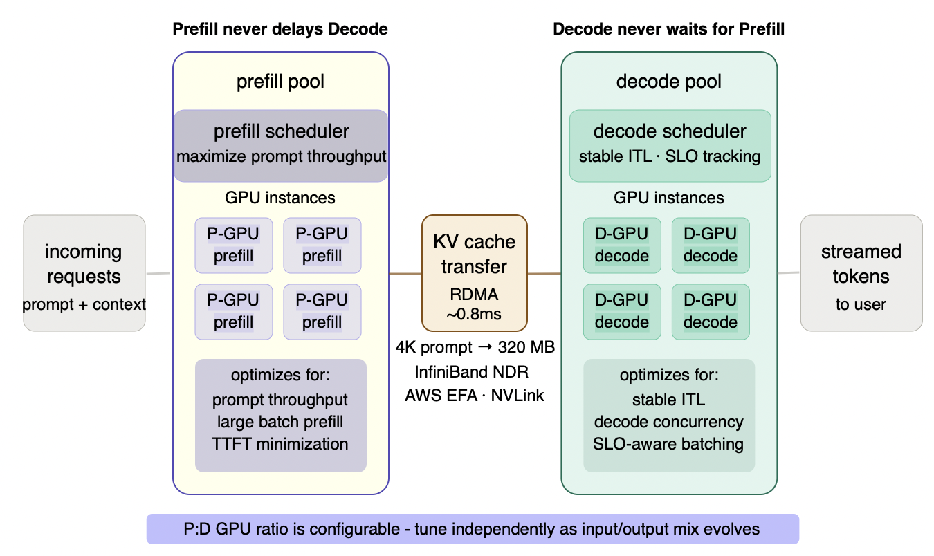
Figure 6.5 - Disaggregated prefill-decode architecture
Incoming requests flow into the prefill pool, which executes the full prompt processing pass and transfers the resulting KV cache via RDMA to the decode pool. From that point, the decode pool handles all token generation independently - no prefill activity ever touches the decode execution path again. Each pool has its own scheduler optimizing for different objectives: the prefill scheduler maximizes prompt throughput and minimizes TTFT; the decode scheduler maintains stable ITL and tracks per-request SLOs. In a colocated system these objectives conflict on every forward pass. Disaggregation makes them independent. The P:D ratio - how many GPUs each pool gets - is configurable and re-tunable as your workload mix evolves. A colocated deployment is permanently fixed at 1:1 regardless of whether your workload is prefill-heavy or decode-heavy.
6.6 Speculative Decoding: Breaking the Decode Bandwidth Ceiling
Every batching strategy in this section - continuous batching, chunked prefill, disaggregation - improves how requests are scheduled and phased. None of them address a more fundamental constraint: during decode, the GPU generates exactly one token per forward pass, loading the full model weights from HBM on every step. At small batch sizes, CUDA cores sit largely idle while the memory subsystem does the work. The roofline model from Section 3 makes this explicit - decode is memory-bandwidth-bound, not compute-bound, and no scheduling optimization changes that.
Speculative decoding attacks this constraint directly by changing what gets fed into the target model's decode step.
Step 1 - Draft model speculates ahead. A small fast draft model (typically 1-3B parameters) runs 4-8 cheap decode steps autoregressively, generating candidate tokens [t1, t2, t3, t4, t5] along with their probability distributions q(t1..t5) from its own weights and KV cache.
Step 2 - Target model verifies in one parallel pass. Normally, the target model's prefill stage produces one token which is fed back into decode as the next input - one token in, one token out, repeat. Speculative decoding replaces that single token input with the draft model's 5 candidate tokens fed in together. The target model processes all 5 simultaneously - extending its existing KV cache with keys and values for all 5 positions in one parallel pass - and produces its own probability distributions p(t1..t5) for each position. Because multiple token positions are processed in parallel, this pass runs compute-bound rather than memory-bandwidth-bound - exactly the roofline shift described in Section 3.
Step 3 - Token acceptance via probability comparison. For each position, the target model compares its distribution against the draft model's. Where they agree, the token is accepted. Where they first diverge, that position and everything after it is rejected and the KV cache rolls back. The target model samples a corrected token from its own distribution at that position - using probabilities already computed during the verification pass, at no extra cost. Worst case - every draft token rejected - you still get one corrected token from one forward pass, identical to vanilla decode. You never do worse than baseline.
The gain is not that the forward pass gets cheaper - the target model still loads all its weights from HBM on every verification pass. The gain is in tokens produced per forward pass. Vanilla decode: one weight-loading trip → one token out. Speculative decoding: one weight-loading trip → three or four tokens out on average. The memory bandwidth cost is amortized across multiple accepted tokens. Think of it as a delivery truck making the same warehouse trip but dropping packages at four houses instead of one - same trip cost, four times the useful work. The output distribution is mathematically identical to what the target model would have produced alone - speculative decoding is lossless, not an approximation.
What this means on the roofline. Speculative decoding shifts decode from the memory-bandwidth-bound regime toward the compute-bound regime by batching multiple token verifications into a single pass. GPU compute utilization during decode - which typically sits at 20-30% for single-token autoregressive generation - rises meaningfully with speculation. With 3-4 tokens accepted per verification pass, the effective arithmetic intensity increases by the same factor, pushing utilization from the 20-30% range toward 60-80% at typical acceptance rates. This is not a full escape from the memory-bandwidth-bound regime but a meaningful shift up the roofline slope.
Acceptance rate is the critical variable. If the draft model's token distribution closely matches the target model's, acceptance rates of 70-90% per token are achievable, yielding 2-4× speedups on latency-sensitive workloads. If the draft model is poorly matched to the domain or the target model's distribution, acceptance rates drop and speculative decoding becomes slower than vanilla autoregressive generation - you pay the overhead of running the draft model without the benefit. Always measure acceptance rate in production; it is the metric that tells you whether speculative decoding is helping or hurting.
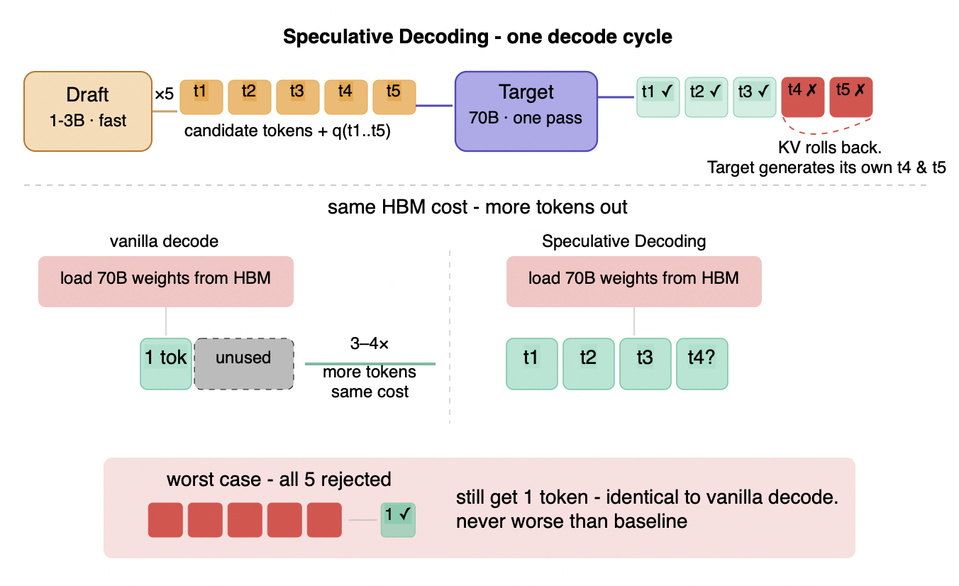
Figure 6.6 - Speculative decoding: mechanism and HBM amortization
Top: the draft model runs 5 cheap autoregressive steps producing candidate tokens. The target model verifies all 5 in one parallel pass - t1, t2, t3 accepted; t4 diverges triggering a rollback to t3 and sampling a corrected t4 from the target's own distribution. Result: 3 tokens from one target model forward pass. Middle: the gain is purely amortization - the same HBM cost of loading all model weights produces 1 token in vanilla decode and 3-4 tokens in speculative decoding. Bottom: worst case guarantees the floor - even if all draft tokens are rejected, you still get 1 corrected token, identical to vanilla decode. The output distribution is mathematically identical to the target model alone.
Three deployment patterns in production:
- Separate draft + target models - a small model (1-3B parameters) runs alongside the large model. Works best when a purpose-trained draft model exists for the target model family. Llama-3 8B as draft for Llama-3 70B is a common pairing. One memory implication worth calculating before deployment: a 3B draft model at FP16 adds 6 GB alongside the target model - modest relative to a 70B target but not free. In memory-constrained configurations, prefer N-gram speculation or EAGLE draft heads instead.
- N-gram speculation - uses n-gram matching on the prompt and previous outputs to generate draft tokens without a separate model. Zero additional memory cost, effective for repetitive or structured outputs (code, templates, JSON). Supported natively in vLLM and SGLang.
- EAGLE / Medusa (draft heads) - adds lightweight prediction heads to the target model itself, trained to speculate future tokens. Higher acceptance rates than separate draft models for matched domains; requires fine-tuning the draft heads on your target distribution.
When speculative decoding helps and when it does not:
| Scenario | Verdict | Reason |
|---|---|---|
| Low-to-medium concurrency, latency-sensitive | High impact | Memory bandwidth is the clear bottleneck; speculation raises arithmetic intensity |
| High concurrency, throughput-optimized | Low or negative impact | At large batch sizes decode becomes more compute-bound; speculation overhead hurts |
| Repetitive or structured output (code, JSON) | High impact | N-gram speculation achieves high acceptance rates at near-zero overhead |
| Creative or highly variable output | Lower impact | Draft model acceptance rates drop; measure before committing |
| Mixed concurrency with variable output length | Measure first | Acceptance rate variance across request types makes aggregate impact unpredictable - benchmark on your actual workload distribution before committing |
| Disaggregated P/D deployment | Compatible | Speculation runs on decode instances independently; prefill instances unaffected |
The strategies in this section are not mutually exclusive - continuous batching, chunked prefill, disaggregation, and speculative decoding compose together. The next section provides the decision framework for which combination makes sense for your specific workload profile.
6.7 Choosing the Right Strategy
The strategies in this section are additive, not mutually exclusive. Continuous batching is always the foundation. Chunked prefill and SLO-aware scheduling layer on top for mixed workloads. Disaggregation is the architectural escalation for large fleets with strict, independent latency targets.
| Scenario | Strategy | When to move up |
|---|---|---|
| Single GPU or small fleet | Continuous batching, FCFS scheduler | P99 ITL spikes appear under mixed input lengths - short requests stalling behind long prompts |
| Mixed workload, variable prompt lengths | + Chunked prefill, SLO-aware scheduler | TTFT and ITL SLOs are independently defined and both need to be met simultaneously |
| Low-to-medium concurrency, latency-critical | + Speculative decoding | Acceptance rate stays above 60% on your workload; memory bandwidth is still the decode bottleneck |
| Large fleet, strict independent SLOs for TTFT and ITL | + Full P/D disaggregation, KV-aware routing | Colocated chunked prefill cannot meet both TTFT and ITL targets simultaneously at peak load |
| Offline batch only | Maximum batch size, FCFS acceptable | N/A - throughput is the only metric; latency SLOs do not apply |