8 · The Latency-Throughput Curve: Finding Your Operating Point
Every optimization covered in this guide - quantization, batching strategy, parallelism, KV cache tuning - ultimately manifests as a shift in one empirical artifact: the latency-throughput curve for your specific model, hardware, and workload. This is where everything comes together. The curve is not theoretical - it is the empirical basis for every fleet sizing decision, SLO definition, and capacity planning conversation you will have in production.
8.1 The Shape of the Curve and Why the Knee Matters
As concurrency increases, throughput and latency evolve differently. Throughput rises rapidly at first as the system utilizes compute and memory bandwidth more efficiently. Latency remains relatively stable during this phase - requests complete quickly because the system has headroom. As concurrency approaches saturation, something changes: latency begins rising sharply while throughput gains flatten. The system is now spending a growing fraction of its time managing queuing, batching overhead, and resource contention rather than doing useful work.
This shape is not LLM-specific - it is a direct consequence of queueing theory. Any system with finite resources exhibits it. What makes LLM inference distinctive is the steepness of the latency climb past the inflection point, driven by the interaction between prefill compute saturation, decode memory bandwidth limits, and KV cache pressure all converging simultaneously.
The inflection point - where latency begins rising faster than throughput improves - is the knee of the curve. In practice the knee is visible in your monitoring dashboard as the concurrency level where P99 TTFT begins diverging from P50 TTFT. When P50 and P99 track closely together, the system is in the safe operating zone. When P99 starts climbing while P50 stays relatively flat, you are at or past the knee - tail requests are queueing while median requests still complete normally. The knee is not a precise point but a region, and its location shifts with workload characteristics, batch size, and the optimizations you have applied.
Beyond the knee, in the saturation zone, every additional concurrent request buys marginal throughput at a steep latency cost. The system has not broken - it is still serving requests - but the economics have inverted. You are paying in user experience for throughput gains that diminish with every additional request added.
Operating beyond the knee is not just inefficient - it is unstable. Small increases in traffic produce disproportionate latency spikes in the saturation regime. A 10% traffic increase that would be invisible in the safe zone can push P99 TTFT from 500ms to 2 seconds past the knee. This is why headroom matters: you are not sizing for average traffic, you are sizing for the worst-case burst that your SLO must survive without crossing into saturation.
The production operating point should sit to the left of the knee, with enough margin to absorb traffic spikes. How much margin depends on your traffic variability - a workload with predictable diurnal patterns needs less headroom than one with unpredictable burst events. Section 1's P95 vs average RPS guidance is directly relevant here: if your P95 RPS is 2.5× your average, your safe operating point must be at least 2.5× below the knee's RPS level.
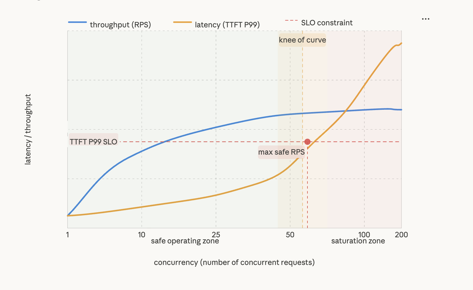
Figure 8.1 - The latency-throughput curve: finding the knee
Throughput (blue) and P99 TTFT latency (amber) respond differently as concurrency increases. In the safe operating zone (left of the knee), throughput grows rapidly while latency stays relatively flat - the system is efficiently utilizing compute and memory bandwidth. At the knee (~60 concurrent requests here), latency begins climbing steeply while throughput gains flatten. Beyond the knee, in the saturation zone, every additional request buys marginal throughput at a steep latency cost as queueing dominates. The red dot marks max safe RPS - the highest concurrency at which P99 TTFT still meets the SLO constraint. This is the production operating point. Sizing the fleet to keep peak traffic to the left of this point - with headroom for spikes - is the central fleet sizing decision.
Understanding the shape of the curve is the first step. Generating it accurately for your specific deployment - model, hardware, workload distribution, and full optimization stack - is the second.
8.2 How to Generate the Curve
The latency-throughput curve cannot be calculated from a formula - it must be measured. Too many variables interact in non-linear ways: KV cache pressure, prefill/decode interference, batching dynamics, and queuing behavior all combine differently at different concurrency levels. The measurement procedure is a concurrency sweep: start at 1 concurrent request, step up to beyond the knee, and record P50 and P99 TTFT, ITL, RPS, and tokens/sec at each step.
Use realistic request distributions, not synthetic uniform load.
This is the single most common mistake in LLM benchmarking. Running a sweep where every request has the same input length and the same output length is like load testing a highway by only sending identical compact cars at uniform spacing. The highway looks fine. Then real traffic arrives - trucks, buses, cars stopping suddenly - and the knee appears much earlier than your benchmark predicted.
Real workloads have heavy-tailed input length distributions. Your P99 input is typically 3-5× your P50 input, and those long-tail requests consume disproportionate KV cache and prefill compute. A sweep measured at uniform 512-token inputs will show a knee at a higher concurrency than your production system actually sustains. Size from your P99 curve, not your P50 curve.
Generate curves for your actual workload archetypes.
There is not one curve for your deployment - there is a family of them, one per input/output length combination. The curve for a RAG workload at 4K input / 200 output looks completely different from a code generation workload at 200 input / 3K output on identical hardware. At minimum generate curves for your P50 and P99 input/output length combinations. If you have multiple workload types on the same fleet, generate one per type.
Also test burst behavior, not just steady-state ramp.
A gradual concurrency ramp shows how the system behaves when load increases slowly. It does not show what happens when 3× normal traffic hits simultaneously - which is exactly what happens during peak events. Run a step-function burst test: send a sudden 2-3× load spike and measure how long TTFT takes to recover. If it takes more than a few seconds to stabilize, your headroom margin is not enough.
Lock down your variables before you start.
A curve is only useful if it is reproducible and comparable. Before running any sweep, explicitly record: model and quantization format, parallelism configuration, hardware, framework version, and input/output length distribution. Benchmark results without these details cannot be used for fleet sizing - they are just numbers without context. This sounds obvious but benchmarks shared without version numbers or length distributions are common and nearly useless.
Always warm up first.
The first few hundred requests in any sweep will show artificially elevated TTFT due to cold KV cache and CUDA initialization. Run at least 1,000 warmup requests and verify TTFT has stabilized before recording measurements.
Tooling.
NVIDIA AIPerf - the successor to GenAI-Perf - supports any OpenAI-compatible endpoint and measures TTFT, ITL, tokens/sec, and RPS directly with configurable concurrency sweeps and length distributions. It is the right starting point for NVIDIA hardware. Watch specifically for where P99 TTFT begins diverging from P50 TTFT - that divergence is the empirical knee, more reliable than looking at throughput alone.
For non-NVIDIA stacks, Locust and k6 work but require custom instrumentation. Standard HTTP response time is not sufficient - you need token-level timestamps for TTFT and ITL specifically, which requires streaming response handling in your load test client.
8.3 From Benchmark to Fleet Size
With the curve in hand, fleet sizing becomes a mechanical process - not an estimate, not a rule of thumb, but a direct calculation from measured data.
The curve gives you two numbers at every concurrency level: latency and throughput. The SLO converts those two numbers into one decision.
Step 1 - Find your SLO-constrained concurrency. On your latency curve, find where TTFT P99 crosses your SLO threshold - say 2 seconds. That concurrency level is C_max: the highest load your instance can sustain without violating the latency budget. Everything to the right is the region where you are technically serving requests but breaking your SLO at the tail.
Step 2 - Read per-instance RPS at C_max. Look at the throughput curve at the same concurrency. That value - not the peak throughput the curve ever reaches - is your usable RPS per instance. The distinction matters: the system may be capable of higher throughput at higher concurrency, but that throughput comes with latency you have agreed not to deliver.
Step 3 - Size the fleet.
instances = ceil(peak_RPS / usable_RPS_per_instance)
total_GPUs = instances × TP_degree × safety_factor
Add a safety buffer of 20-50% on top of the calculated capacity. This is not conservative padding - it accounts for real-world conditions. Peak traffic estimates are usually based on P95 and are routinely exceeded. Rolling restarts temporarily take instances offline. Operating exactly at C_max leaves no margin - any variability such as longer prompts, cache misses, or scheduling delays can push the system into SLO violations. Use 20% for stable, predictable workloads with well-understood traffic patterns. Use 50% for new deployments without historical traffic data, workloads with high input length variance, or any deployment where an SLO violation is operationally severe.
The failure mode to avoid. The most common capacity planning mistake is sizing for average throughput - what the system delivers at P50 - rather than SLO-constrained throughput at C_max. The result is a system that looks healthy on dashboards, passes load tests at average traffic, and then violates P99 SLOs during peak hours - exactly when failures are most visible and most costly. The curve makes this failure mode visible before it reaches production. Little's Law gives you the sanity check to confirm your benchmark is actually telling you the truth about production conditions.
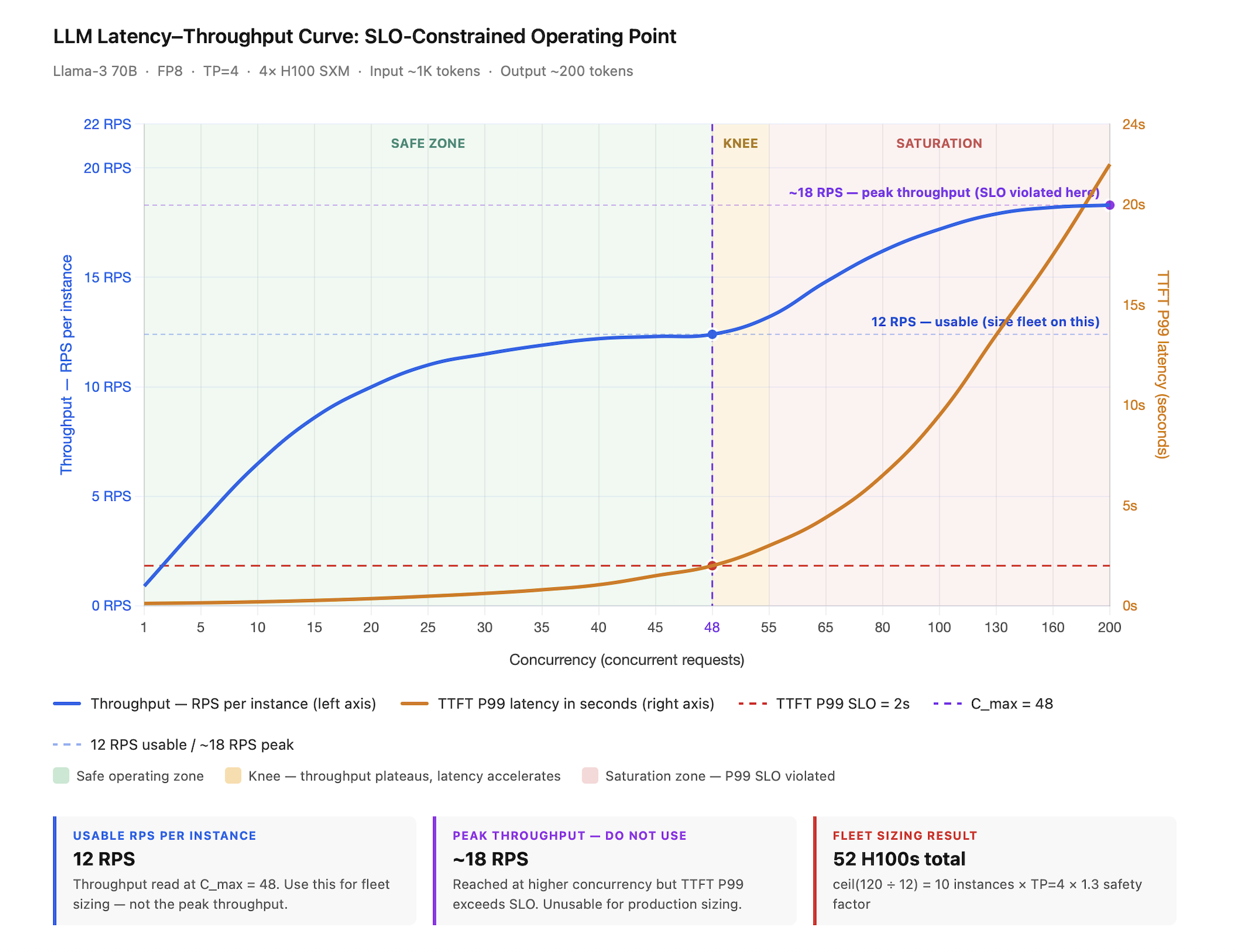
Figure 8.2 - SLO-constrained operating point: from benchmark to fleet size
Llama-3 70B · FP8 · TP=4 · 4× H100 SXM · ~1K input / ~200 output tokens. The TTFT P99 SLO of 2s (red dashed line) intersects the latency curve at C_max = 48 concurrent requests (purple dashed line) - this is the hard ceiling. Everything to the right is the saturation zone where the system is technically serving requests but breaking the latency contract at the tail. Reading throughput at C_max gives 12 RPS usable per instance - not the ~18 RPS peak the curve eventually reaches, which is unreachable without SLO violation. Fleet sizing follows directly: ceil(120 peak RPS ÷ 12 usable RPS) = 10 instances × TP=4 × 1.3 safety factor = 52 H100s total. The gap between the 12 RPS measured and the 24 RPS theoretical ceiling (C_max ÷ SLO = 48 ÷ 2) is expected - the theoretical formula assumes every request takes exactly 2s, while real traffic has variable prompt lengths, cache misses, and scheduling overhead. A gap under 2× means the benchmark reflects production conditions well. A gap over 2× means the benchmark inputs are wrong and the fleet will be under-provisioned.
Sanity check with Little's Law. Little's Law gives you a theoretical ceiling to validate your benchmark against:
maximum_sustainable_RPS = C_max ÷ average latency
Plugging in the example: at C_max = 48 and a 2s SLO, the theoretical ceiling is 48 ÷ 2 = 24 RPS. The benchmark measured 12 RPS - roughly half.
That gap is not a problem. It is expected. The theoretical formula assumes every request takes exactly 2s. In reality, some requests are longer, some shorter, and the system spends real time on scheduling, KV cache management, and prefill interference. The 24 RPS ceiling is the best case; 12 RPS is what you actually get after system overhead.
Use the gap as a calibration signal. If the gap is under 2×, your benchmark reflects production conditions well and you can proceed with sizing. If the gap exceeds 2×, your benchmark inputs do not match production - the most common cause is test prompt lengths or arrival patterns that differ from real traffic. Fix the benchmark before sizing the fleet. A fleet sized from a mismatched benchmark will be under-provisioned, and the under-provisioning will only surface during peak hours when it is most costly to discover.
Why operating beyond the ceiling always fails. Once the arrival rate exceeds C_max ÷ average latency, the system cannot process requests fast enough. The only way it re-establishes balance is by letting latency grow - requests wait longer, the equation rebalances at a higher latency. This is not a bug. It is a mathematical property of any queuing system. You cannot run past this ceiling without breaking your SLO. Sizing from C_max is how you enforce that ceiling proactively.
8.4 Start With the Question, Not the Metric
Fleet sizing tells you how many instances you need. The metric you use to track and compare performance determines whether you are measuring the right thing - and the wrong metric is one of the most common sources of misleading benchmark comparisons and bad procurement decisions.
The instinct when evaluating system performance is to lead with metrics - tokens/sec, RPS, utilization - and then work backward to conclusions. This gets the direction wrong. The right approach is to start with the business or operational question you are actually trying to answer, then identify which metric answers it precisely. The same system can look excellent on one metric and poor on another - not because the system changed, but because the question changed. Using tokens/sec/GPU to answer a cost efficiency question will give you a number that looks reasonable and leads you to the wrong fleet size.
Think of it like measuring a delivery service. If your question is "how fast are my trucks?" you measure speed. If your question is "how much am I spending per package delivered?" you measure cost per delivery. If your question is "are my customers receiving packages on time?" you measure on-time delivery rate. All three use the same trucks and the same routes - but the metric changes completely based on what you need to know. The same principle applies here.
One rule that applies across every row in the table below: never report any metric without also reporting the input/output length distribution it was measured at. A tokens/sec/GPU number at 128-token inputs is not comparable to one at 4K inputs on identical hardware. Vendor benchmark numbers and framework comparison posts routinely omit input/output length distributions - which means the headline tokens/sec figure tells you how fast the system ran on someone else's workload, not yours. Always verify what length distribution a published benchmark used before drawing any conclusions for your deployment.
| Business / Operational Question | Why it matters | Metrics that answer it |
|---|---|---|
| Is my hardware being used efficiently? | Determines whether optimization headroom exists before buying more GPUs - low efficiency means software changes can still help; high efficiency means hardware is the only remaining lever | MFU (Model FLOP Utilization) - ratio of achieved to theoretical peak FLOP/s. Tokens/sec/GPU - strips out instance count and parallelism degree for pure hardware efficiency comparison across frameworks or quantization strategies |
| Am I serving users within my latency contract? | The only question that directly maps to user experience and SLO compliance - throughput without this is meaningless | Goodput (SLO-compliant RPS) - counts only requests completed within SLO. A system serving more requests but violating more SLOs has high throughput and low goodput. Always track alongside raw RPS. TTFT P99 and ITL P99 - the latency dimensions of the SLO contract |
| How many requests can each routing unit handle? | Determines autoscaling thresholds and load balancer configuration - your load balancer routes to instances, not GPUs | RPS/instance - the unit your infrastructure actually scales and routes on. Tokens/sec/GPU is invisible to your load balancer |
| What am I getting per dollar of GPU spend? | The cost efficiency question for fleet sizing and procurement - collapses hardware configuration into a single comparable number | RPS/GPU - collapses TP degree and instance count into a cost-normalized figure. A TP=2 deployment may beat TP=8 on RPS/instance but lose on RPS/GPU once you account for GPU count. TTFT per dollar - adds the latency dimension to cost, essential when comparing GPU generations or cloud providers where price-per-GPU differs |
| How much of my capacity is doing useful work right now? | Real-time operational question - the leading indicator of approaching the knee before latency metrics start moving. By the time TTFT rises, you are already past the knee | Queue depth and concurrency utilization - move before latency moves, giving you advance warning. GPU utilization - distinguishes between GPU idle (system under-loaded) and GPU busy but inefficient (wrong bottleneck, e.g. memory-bound decode with idle CUDA cores) |
| Is my system bottlenecked on decode or prefill? | Determines which optimization lever to reach for - decode bottleneck calls for larger batch sizes, higher bandwidth, or speculative decoding; prefill bottleneck calls for more compute or chunked prefill | TTFT vs ITL ratio - high TTFT relative to ITL signals prefill is the bottleneck; high ITL relative to TTFT signals decode. Output tokens/sec vs input tokens/sec ratio - a system spending most time on decode shows disproportionately high cost per output token relative to input token |
| How efficiently am I using my memory budget? | Relevant when KV cache dominates - long contexts, high concurrency, or when evaluating quantization strategies for memory impact | Tokens/sec per GB HBM - captures the memory efficiency dimension that tokens/sec/GPU misses at long contexts. KV cache utilization - what fraction of allocated KV memory is actively used versus fragmented or empty |
| Is my benchmark representative of production? | Determines whether fleet sizing from the benchmark will be accurate or systematically wrong - a mismatched benchmark produces a fleet that under-provisions exactly at peak load | Little's Law gap - compare your measured benchmark RPS against the theoretical ceiling of C_max ÷ average latency. Gap under 2× means the benchmark reflects production conditions. Gap over 2× means your test inputs do not match real traffic - fix the benchmark before sizing the fleet |
| How do I compare two hardware or framework configurations fairly? | Procurement and architecture decisions require apples-to-apples comparisons - most public benchmarks fail this test | Tokens/sec/GPU at matched input/output length distributions and matched batch size. Any comparison that does not hold these variables fixed is comparing different workloads, not different hardware. Always report the full configuration alongside the number |
The metrics above tell you the current state of your system. What they do not tell you is how a specific optimization - quantization, batching strategy change, parallelism reconfiguration - shifts the curve itself. That is what Section 8.5 covers.
8.5 How Optimizations Shift the Curve
Tracking the right metrics tells you where you are on the curve. This section tells you which lever moves it - and in which direction.
Without the curve, optimization decisions are guesses. With it, every lever has a predictable, measurable effect. Apply an optimization, re-benchmark, and the curve tells you whether it worked and by how much. If the curve did not shift in the expected direction, something else is the binding constraint - and the curve tells you that too.
| Optimization | Effect on curve | When to reach for it | What it does not fix |
|---|---|---|---|
| Continuous batching | The single largest curve shift available - moves the knee dramatically rightward by eliminating idle GPU slots between requests. Transforms ~55% GPU utilization to ~95% on the same hardware. Non-negotiable baseline. | Every deployment. If your serving stack does not support it, no other optimization in this table is as effective. | Does not address the prefill/decode interference problem - KV cache pressure and ITL spikes under mixed loads remain. |
| PagedAttention | Shifts the curve right by eliminating the 20-38% memory waste from contiguous KV allocation. Increases the concurrency the system sustains before hitting the memory ceiling without adding hardware. | Every deployment - it is the default in all major frameworks. If you are not using it, you are wasting your KV cache budget. | Does not solve cross-GPU memory imbalance in TP deployments - the most memory-pressured GPU is still the bottleneck. |
| Quantization (FP16 → FP8) | Shifts the entire curve right - more RPS at the same latency, or same RPS at lower latency. Knee moves right too, so you can sustain higher concurrency before saturation. | GPU memory is the binding constraint; you need more concurrent requests per GPU without adding hardware. | Does not help if your bottleneck is compute saturation rather than memory capacity. |
| Model routing / cascading | Does not shift the large model's curve - reduces traffic volume reaching it. The large model fleet operates at lower effective RPS, moving your operating point left on its curve and improving utilization headroom. | Traffic has measurable complexity skew - many simple requests a smaller model handles adequately. Large model fleet exceeds 8 GPUs. | Does not improve large model latency or throughput. Adds router latency (5-20ms). Misclassification degrades quality on complex requests routed to the small model. |
| Multi-LoRA serving | No direct effect on curve shape - the base model performance is unchanged. The effect is on fleet economics: one GPU fleet serves N fine-tuned variants instead of N separate fleets, dramatically improving fleet utilization and reducing total GPU count. | Serving multiple fine-tuned variants of the same base model for different tenants or use cases. Without Multi-LoRA you would need a separate fleet per variant. | Does not improve latency or throughput for any individual variant. If simultaneous adapter count exceeds GPU memory budget, adapter paging adds latency that looks like prefill interference but has a different cause. |
| Speculative decoding | Lowers ITL at low-to-medium concurrency by producing multiple tokens per target model forward pass - extends the flat latency region leftward. No effect on peak RPS. At high concurrency the curve can worsen as verification overhead compounds. | Latency-sensitive workloads at low-to-medium concurrency where decode ITL is the bottleneck and a suitable draft model or n-gram pattern exists. | Does not help at high concurrency or throughput-dominated workloads. Acceptance rate must be measured - a poor draft model match makes it slower than vanilla decode. |
| KV cache quantization (FP8/INT8 KV) | Independently shifts the curve right by increasing the number of concurrent requests that fit in GPU memory - orthogonal to model weight quantization. | High concurrency workloads where KV cache is the memory ceiling, not model weights. | Does not reduce per-token compute cost. |
| KV cache offloading | Extends the concurrency range beyond what GPU HBM alone supports by tiering cold KV blocks to CPU DRAM or NVMe. Trades a latency floor increase for offloaded requests in exchange for higher total concurrency. | Long-context batch workloads where KV cache structurally exceeds GPU HBM capacity. Not suitable for interactive workloads. | Adds 125ms+ reload latency per cache miss from CPU DRAM. NVMe tier adds ~1s per miss - only viable for offline batch with no interactive SLO. |
| KV cache eviction policy | Right policy maintains prefix cache hit rate under memory pressure, preventing TTFT curve degradation as load increases. Wrong policy causes hit rate collapse under load, which appears as a curve shape change rather than a capacity problem. | Any deployment relying on prefix caching at high utilization. LRU is the right default; switch to frequency-based if high-frequency prefixes are repeatedly evicted. | Does not increase total KV cache capacity - it only determines which entries survive when capacity is exhausted. |
| Prefix caching (high hit rate) | Compresses the effective TTFT curve downward for cache-hit requests - extends the flat latency region significantly. Does not change peak throughput but dramatically improves perceived latency at the same concurrency. | Workloads with shared system prompts, RAG context, or repeated prefixes - multi-turn chat, agentic pipelines. | No benefit for workloads where every request has a unique prefix. Cache hit rate must be measured - assumed hit rates are unreliable. |
| Cache-aware routing | Restores prefix cache hit rate in multi-replica deployments - without it, round-robin routing collapses hit rate to ~1/N regardless of cache configuration. Enables the prefix caching curve benefit to survive horizontal scaling. | Any multi-replica deployment relying on prefix caching for TTFT improvement. Single-instance deployments do not need it. | Does not help if your workload has no prefix reuse. Creates load imbalance risk if popular prefixes concentrate traffic on one replica. |
| SLO-aware scheduling | Does not shift the curve itself - changes which requests operate in the flat region versus the saturation region. Protects high-priority requests from tail latency degradation while allowing lower-priority traffic to absorb saturation. | Mixed workloads with different latency classes - interactive chat, batch summarization, and RAG pipelines sharing a fleet. | Does not increase overall capacity. A system at full saturation violates SLOs regardless of scheduling policy. |
| Chunked prefill | Flattens the ITL curve under mixed workloads - reduces the latency spikes that appear when large prefills enter the batch. Does not increase peak RPS but stabilizes the shape of the curve. | ITL P99 is violating SLO under mixed input lengths even though average ITL is fine. | Does not help TTFT - may slightly increase TTFT for the chunked request itself since prefill is spread across iterations. |
| P/D disaggregation | Replaces one curve with two independent curves - one for prefill, one for decode - each with its own knee and SLO operating point. Allows each phase to be sized and optimized independently. | Large fleet with strict, independent TTFT and ITL SLOs that cannot both be met on a colocated system. | Adds operational complexity and KV transfer overhead. Net negative for short prompts where transfer cost exceeds interference savings. |
| Data parallelism (horizontal scaling) | Duplicates the curve horizontally - multiplies peak RPS linearly with replica count at zero latency overhead. The cleanest scaling lever: doubles replicas, doubles capacity, no tradeoffs. | Per-instance performance is already optimized and you need more aggregate throughput. The last lever to reach for, not the first. | Does not improve per-instance latency or throughput. Each replica must hold a complete model copy - does not reduce per-GPU memory requirements. |
| Larger TP degree | Lowers per-request latency at low concurrency by parallelizing computation across more GPUs. At high concurrency, all-reduce overhead grows and the knee moves left per replica - you reach saturation earlier with fewer replicas available to absorb traffic spikes. | Latency-sensitive workloads at low to medium concurrency where TTFT or ITL is the binding constraint. | Reduces RPS/GPU - more GPUs per instance means fewer replicas for the same hardware budget. Verify RPS/GPU does not regress. |
| Expert parallelism (MoE models) | For MoE architectures, EP enables serving models that would not otherwise fit on available hardware, shifting the curve from non-existent to viable. At scale, Wide-EP improves throughput by distributing expert routing across a larger GPU pool. | Any MoE model deployment at scale. For DeepSeek-V3 class models, EP is not optional - it is the mechanism that makes the economics viable. | All-to-all communication overhead adds latency that does not compress well. EP is primarily a throughput optimization, not a latency optimization. Hot expert imbalance can cap throughput well below theoretical maximum. |
| Higher input/output length | Shifts the entire curve left - lower RPS per GPU, earlier saturation, and steeper latency rise. Not an optimization but a workload reality that must be accounted for in sizing. | N/A - this is a workload characteristic, not a lever. Re-benchmark when your input/output distribution changes materially. | Nothing fixes this except more hardware or a smaller/quantized model. |
How to use this table in practice. Start from your specific symptom on the curve, not from a list of optimizations to apply:
- TTFT too high at low concurrency → check prefix cache hit rate first, then TP degree
- ITL spikes under mixed load → chunked prefill is the first intervention
- Throughput plateau too low → quantization (model weights + KV cache) before adding hardware
- Cannot meet TTFT and ITL SLOs simultaneously → P/D disaggregation
- RPS/GPU degrading as you scale TP → you have passed the all-reduce crossover point; reduce TP and add replicas instead
- ITL too high at low concurrency with low GPU compute utilization → speculative decoding before reaching for more hardware
- TTFT spikes on specific tenants but not others, with no prefill pattern → check adapter cache eviction rate; an evicted LoRA adapter being paged back from CPU is the likely cause
- P99 latency healthy at low load but spikes at peak → you are operating too close to the knee; increase fleet size or apply quantization to move the knee right before the next peak event
The optimizations and levers above address individual components of the system. Section 9 puts them together into a complete sizing algorithm - a sequenced decision process that takes you from workload characterization to a production-ready fleet configuration.