4 · Quantization: Trading Precision for Scale
Section 3 established that quantization affects prefill and decode differently - halving memory bandwidth pressure for decode while primarily freeing VRAM capacity for prefill. Before examining those phase-specific effects, the foundation is the memory arithmetic, because that is where the leverage is most visible.
Neural network weights follow smooth, well-behaved distributions clustered around zero. Representing each weight as a 16-bit float when an 8-bit or 4-bit integer captures nearly the same information is like printing a temperature forecast to six decimal places - the extra precision costs memory and bandwidth without meaningfully changing the answer. The practical stakes are significant: Llama-3 70B at FP16 requires 140 GB for weights alone. The same model at INT4 requires 35 GB - the difference between a multi-node setup and a single 8-GPU node with room left for KV cache. At production scale, quantization is not a compromise for resource-constrained environments. It is the standard operating mode.
No other single optimization lever simultaneously reduces model weight memory, shrinks KV cache footprint, increases HBM bandwidth efficiency, and improves decode throughput - without changing model architecture or retraining from scratch. The sections that follow examine each of these effects in turn.
4.1 Weight-Only Quantization: Compress the Model, Keep Everything Else
Weight-only quantization compresses the static model weight matrices while leaving activations and KV cache at higher precision. Think of it like compressing a large file before transmission - the weights are stored and loaded in compressed form, then decompressed for computation. The KV cache and runtime activations are unaffected.
Three formats dominate production deployments:
GPTQ (Generalized Post-Training Quantization) compresses model weights to lower precision by solving for the quantized values that best preserve what each layer actually produces - not just what individual weights look like in isolation. This distinction matters. Naive quantization rounds each weight independently to the nearest representable lower-precision value. GPTQ does something smarter: it runs a small representative sample of real inputs - called a calibration dataset - through the model, observes how each layer transforms those inputs, and then chooses quantized weights that minimize the error in the layer's output rather than the error in the weights themselves.
The optimization runs block by block within each layer. As weights are quantized in each block, GPTQ measures how much the layer's output has drifted from the original and uses that information - specifically a mathematical structure called the Hessian, which captures how sensitive the output is to changes in each weight - to distribute the quantization error as evenly as possible across the remaining weights in the block. Weights that the model is highly sensitive to get quantized more carefully; weights that have little influence on the output absorb more of the rounding error. The result is a quantized model where accumulated output error is minimized globally across each layer, not just locally weight by weight.
No retraining is required - GPTQ runs once after training is complete, typically in a few GPU-hours for a 70B model. It delivers strong output quality even at INT4 and is widely supported across vLLM, TensorRT-LLM, and HuggingFace.
AWQ (Activation-aware Weight Quantization) takes a sharper approach than GPTQ. It starts from an observation: not all weights contribute equally to model output. When a weight is paired with a high-magnitude activation - a large intermediate value flowing through the network - even a small quantization error in that weight gets amplified significantly in the layer's output. AWQ identifies the roughly 1% of weights in this high-sensitivity category and protects them from aggressive quantization, while compressing the remaining 99% more aggressively than it otherwise would. The result is better accuracy than GPTQ at the same bit width, particularly on reasoning and instruction-following tasks, because the weights that actually drive output quality are preserved at higher precision. For production serving at INT4, AWQ is generally the preferred choice.
GGUF, used by llama.cpp, applies mixed-precision quantization per layer and is the standard format for on-device and CPU inference. It is outside the scope of cloud-scale serving covered in this guide but worth knowing for edge deployment scenarios.
The memory impact is straightforward: FP16 to INT8 reduces weight memory by 50% with negligible quality loss on most benchmarks. FP16 to INT4 via AWQ or GPTQ reduces it by 75% - a 1-3% perplexity increase that is generally imperceptible in production chat or RAG workloads but may surface in complex multi-step reasoning chains.
One important caveat: weight-only quantization captures the weight saving entirely but leaves KV cache and activation memory unchanged. At low concurrency this is sufficient - weights dominate the budget. At high concurrency with long context, KV cache grows to match or exceed weight memory, and weight-only quantization captures a shrinking fraction of the total saving. This is why KV cache quantization is a separate lever, covered in the next subsection.
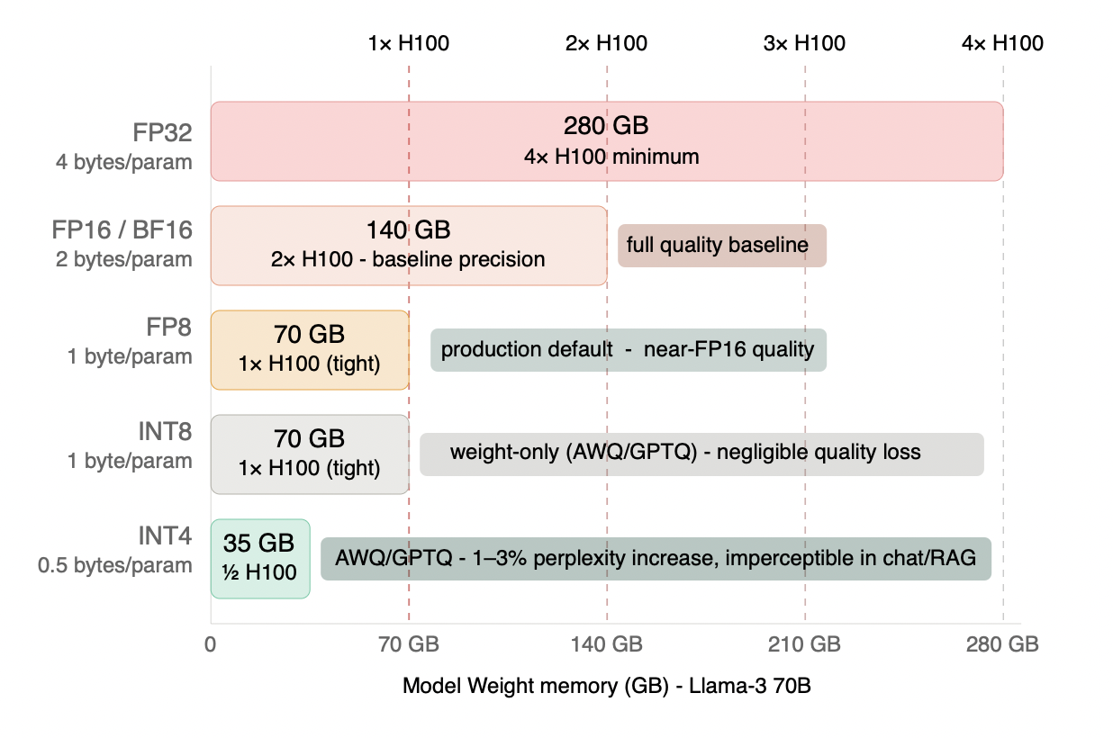
Figure 4.1 - Model weight memory by precision format: Llama-3 70B
Every halving of bit-width halves the weight memory footprint. FP16 to FP8 cuts 140 GB to 70 GB - the difference between needing 2 H100s and fitting on 1. FP16 to INT4 (AWQ/GPTQ) cuts to 35 GB - a 75% reduction with typically imperceptible quality loss for chat and RAG workloads. FP8 is the recommended production default: it unlocks native Tensor Core acceleration on H100 and Blackwell while preserving near-FP16 output quality. Note that these figures cover model weights only - KV cache and activation memory are calculated separately and follow their own precision rules.
4.2 Activation Quantization: Unlock Hardware Acceleration
Weight-only quantization, as covered in the previous section, compresses the weights but leaves activations untouched - and critically, it decompresses weights back to FP16 before the actual matrix multiplication runs. This means the compute path stays in FP16 regardless of how aggressively the weights were compressed. Activation quantization changes this. By keeping both weights and activations in low precision all the way through the computation, it unlocks a different category of hardware capability entirely.
Modern GPUs like the H100 and Blackwell have dedicated hardware units - Tensor Cores - that run INT8 and FP8 matrix multiplications significantly faster than FP16. Weight-only quantization cannot use these faster units because the activations are still in FP16. Activation quantization can. This makes activation quantization a compute throughput lever, not just a memory lever - and that distinction matters for decode-heavy workloads where throughput is the binding constraint.
The catch is that activations are harder to compress than weights. Weights are fixed after training and follow smooth, predictable distributions - they compress cleanly. Activations change with every input, and they regularly produce large outlier values far outside the normal range. Low-bit formats like INT8 struggle here. You can either clip the outliers and lose information, or stretch the representable range to cover them and waste most of your precision on values that rarely occur. Either way, naive INT8 activation quantization hurts model quality noticeably on transformer models.
SmoothQuant gets around this with a neat mathematical trick. If you multiply a weight matrix by some scaling factor S and divide the corresponding activation by the same S, the final output of that layer does not change - the two operations cancel out exactly. SmoothQuant uses this to move the difficulty from activations to weights. It picks scaling factors that shrink activation outliers down to a range INT8 can handle cleanly, and bakes the inverse of those scaling factors into the weights to keep the math identical. This is done once, offline, after training. At inference time, activations are well-behaved and easy to quantize, the weights already carry the compensation, and the output is mathematically equivalent to the original. No retraining needed.
Think of it like balancing a seesaw. If one side is too heavy to fit within a weight limit, you do not remove weight - you slide the fulcrum. The total weight is unchanged, the balance is unchanged, but now both sides sit within the allowed range. SmoothQuant slides the fulcrum between activations and weights so that the activation side - which was too heavy for INT8 - becomes manageable, while the weight side absorbs the shift. The total computation is identical.
The result is a modified set of weights and scaling factors that make activations much smoother and easier to quantize at runtime.
FP8 (W8A8) is where most production systems land today on H100 and Blackwell. The notation is simple: W means weights, A means activations, and the number is the bit width. W8A8 means both weights and activations run in 8-bit precision. You will also see W4A16 - 4-bit weights, 16-bit activations - which is weight-only quantization. This naming convention appears throughout vLLM, TensorRT-LLM, and most inference benchmarks and is worth internalizing.
To understand why FP8 is preferred over INT8 at the same bit width, it helps to think of the three formats as a spectrum. FP16 is accurate but heavy - 2 bytes per value, high memory and bandwidth cost. INT8 is fast and light - 1 byte per value - but uses a fixed-point representation that spreads 256 evenly-spaced values across a fixed range. That works well for weights but is rigid when activations have occasional large spikes, which is the normal condition in transformer inference. FP8 sits deliberately in the middle: it uses floating-point representation like FP16, allocating bits between a range exponent and a precision mantissa, which gives it a much wider dynamic range than INT8 at the same 1-byte storage cost. In practice FP8 handles activation outliers naturally, typically needs no SmoothQuant preprocessing, and preserves near-FP16 output quality. On H100 SXM, FP8 Tensor Cores deliver roughly 2× the throughput of FP16 at equivalent batch sizes - making FP8 W8A8 the default for high-throughput production inference on current hardware.
FP8 W8A8 solves the compute path. The remaining memory problem - the KV cache, which at high concurrency can grow larger than the model weights themselves - has its own quantization lever, and it is the simplest one to apply in practice.
4.3 KV Cache Quantization: The Easiest Win in Production
This is the simplest quantization lever in the stack. Weight quantization requires careful method selection, calibration datasets, and accuracy validation that can take days. KV cache quantization requires almost none of that - in vLLM it is a single startup flag: kv_cache_dtype=fp8. TensorRT-LLM has an equivalent parameter at engine build time. The reason it is so forgiving is that small errors in cached key-value vectors rarely propagate strongly enough to affect final token probabilities in a meaningful way - the attention mechanism is naturally tolerant of small perturbations in the KV vectors.
The payoff is immediate and concrete. Reducing KV cache precision from FP16 to FP8 cuts KV cache memory in half. Half the KV cache memory means you can fit twice as many concurrent requests on the same hardware at the same context length. This is not a traditional throughput optimization - it is a concurrency gain, which translates directly into higher requests per second per GPU without touching the model or changing the system architecture.
Think of it like a warehouse that stores parcels. If you switch from large boxes to smaller ones that hold the same contents, you can fit twice as many parcels in the same space. The parcels - your KV vectors - are slightly less precisely packed, but they still contain everything needed to do the job.
On newer hardware like NVIDIA Blackwell, even more aggressive formats are available. NVFP4 for KV cache reduces memory by another ~50% compared to FP8, with negligible accuracy loss - typically under 1% degradation across long-context and code generation benchmarks. If FP8 doubles your concurrent request capacity over FP16, NVFP4 doubles it again - a 4× concurrency multiplier on Blackwell hardware, from a configuration change alone.
For long-context workloads or high-concurrency serving targets, KV cache quantization is almost always the first optimization to reach for. No retraining, no architecture changes, no calibration pipeline - just a configuration update, a validation run on your target workload, and meaningfully more capacity on the same hardware.
4.4 Sparsity: A Different Dimension of Compression
Quantization reduces how precisely each weight is stored. Sparsity takes a different approach - it removes weights entirely by setting many of them to zero. Think of it like cleaning up a workspace: quantization repacks everything into smaller containers, while sparsity throws away items you do not actually need. Once a weight is zeroed out, the hardware does not have to load or compute it at all.
Modern GPUs like the H100 support a specific pattern called 2:4 structured sparsity - out of every 4 consecutive weights, exactly 2 must be zero. Because this pattern is fixed and predictable, the hardware can skip the zero values during matrix multiplication and deliver up to 2× the compute throughput compared to a dense model of the same size. Tools like SparseGPT can convert a trained dense model into this format without retraining, by identifying which weights can be safely zeroed with minimal impact on output quality.
The practical caveat matters for sizing decisions. The 2× compute speedup from sparsity is most valuable when your workload is compute-bound - large batch prefill, for example. For decode at small batch sizes, the GPU is memory-bandwidth-bound, and removing weights does not help because the bottleneck is data movement, not arithmetic. Sparsity does reduce the number of weights loaded from HBM per step, which provides some memory bandwidth benefit, but the gains are less dramatic than in the compute-bound regime. If your primary bottleneck is decode throughput at low concurrency, sparsity is less impactful than KV cache quantization or batching strategy.
Sparsity and quantization can be combined - a sparse FP8 model benefits from both fewer weights and lower precision per weight. This is increasingly common on H100 and Blackwell for prefill-heavy workloads where maximizing compute throughput is the goal. For most production deployments, the recommended order of operations is: quantize first to FP8, validate quality, then evaluate sparsity if compute throughput remains the binding constraint after quantization.
4.5 Choosing the Right Approach
The four techniques covered in this section are not mutually exclusive - they stack. The question is not which one to use, but in what order and combination for your specific workload. A practical starting rule: begin with KV cache quantization because it requires no accuracy validation and delivers immediate concurrency gains, then layer weight quantization on top if memory or throughput constraints remain. The decision table below maps the most common production scenarios to the right starting point.
| Scenario | Recommendation | Why |
|---|---|---|
| Maximum output quality, VRAM not constrained | FP16 or BF16 (no quantization) | Highest fidelity, no approximation |
| Standard production serving on H100 / Blackwell | FP8 (W8A8) + FP8 KV cache | Best balance of accuracy, throughput, and memory - native Tensor Core support on current hardware |
| Decode-dominated workload, throughput is the bottleneck | FP8 W8A8 + FP8 KV cache + maximize batch size | Decode is memory-bandwidth-bound - FP8 halves bytes moved per step, directly raising the throughput ceiling |
| Memory constrained, quality still important | INT8 weights (AWQ / GPTQ) + FP16 KV cache | Reduces model weight memory while preserving activation and KV cache precision |
| Maximum compression, quality-tolerant workloads (chat, RAG) | INT4 via AWQ + FP8 KV cache | 75% weight memory reduction with typically imperceptible quality loss for chat and RAG workloads |
| Long context or high concurrency is the primary bottleneck | Prioritize KV cache quantization first - FP8, or NVFP4 on Blackwell | Directly halves or quarters KV cache memory, doubling or quadrupling concurrent request capacity |
| Unsure where to start | KV cache quantization before weight quantization | Fastest and safest first step - no calibration, no accuracy validation pipeline, immediate capacity gain |
One column worth internalizing across all rows: the "why" is always rooted in which hardware resource is the binding constraint for your workload. Memory-bound scenarios benefit most from reducing bytes. Compute-bound scenarios benefit most from unlocking faster Tensor Core paths. Matching the technique to the actual bottleneck - rather than applying quantization generically - is what separates a principled sizing decision from a guess.
Quantization addresses the per-GPU memory and compute efficiency problem. The next lever - parallelism strategy - addresses how to scale across multiple GPUs once the single-GPU operating point is optimized.