5 · Parallelism Strategy: Splitting a Model Across GPUs
The single-GPU operating point is now optimized. The next question is what happens when one GPU is not enough - either because the model does not fit in memory, or because a single device cannot meet your throughput targets even when it fits. A 405B model at FP8 requires well over 200 GB - multi-GPU execution is not optional. Even models that fit on one GPU may fall short of RPS targets under production concurrency. Parallelism is how you scale beyond both limits.
There are four primary parallelism strategies for LLM inference. They differ in what they partition, what they optimize for, and the communication overhead they introduce. Choosing the wrong strategy - or the right strategy on the wrong interconnect - can negate the theoretical gains entirely. Tensor Parallelism=4 on PCIe, for example, can deliver worse latency than Tensor Parallelism=2 on NVLink despite using twice the hardware, because the all-reduce overhead consumes more time than the compute saving buys back. The interconnect is not a footnote - it is a first-class input to the parallelism decision.
5.1 Tensor Parallelism: Split the Math, Reduce the Latency
Tensor parallelism splits weight matrices within a layer across GPUs. Each GPU holds a fraction of each weight matrix, computes a partial result on every forward pass, and an all-reduce operation combines those partial results before the computation moves to the next layer. Every GPU participates in every layer of every request.
The benefit is lower latency: each layer's compute is distributed, reducing per-step wall-clock time. TP=4 on a 70B model reduces per-GPU memory to approximately 35 GB and shortens each layer's matrix multiplication proportionally - four GPUs doing a quarter of the work each, in parallel.
The cost is communication. Each layer requires an all-reduce across GPUs, making interconnect bandwidth critical. On NVLink (~900 GB/s), this overhead is modest; on PCIe (~128 GB/s), it can consume 20-30% of step time, significantly reducing the gains. In practice, TP above 2 without NVLink rarely delivers the expected improvement and often makes things worse.
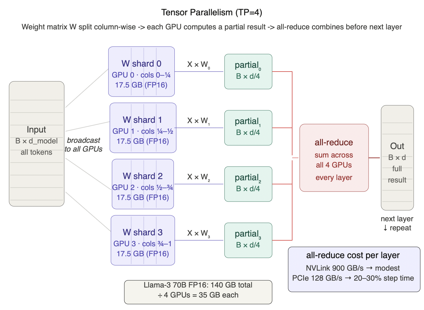
Figure 5.1 - Tensor parallelism (TP=4): one transformer layer
The weight matrix W is split column-wise across 4 GPUs - each GPU holds one quarter of the columns (17.5 GB for Llama-3 70B FP16). All 4 GPUs receive the full input batch simultaneously (broadcast), each computes its partial result independently in parallel, then a single all-reduce sums the four partial outputs before the result passes to the next layer. This repeats at every layer boundary. The memory benefit is immediate - 140 GB drops to 35 GB per GPU. The cost is the all-reduce: trivial on NVLink (900 GB/s) but 20-30% of step time on PCIe (128 GB/s), which is why TP > 2 without NVLink rarely delivers expected latency improvements.
Tensor parallelism also directly reduces the number of independent model replicas per node. At TP=4 on an 8-GPU node you have 2 replicas instead of 8. At TP=8 you have one replica per node - minimum latency, maximum per-request speed, but a single node can handle far fewer concurrent requests than a lower-TP configuration. This is the fundamental tradeoff: TP trades aggregate throughput for per-request latency.
For online serving, use the lowest TP degree that fits the model in memory and meets your per-GPU memory budget. More replicas at lower TP typically deliver higher aggregate throughput. The exception is strict TTFT SLOs - if latency requirements cannot be met by a single GPU at the required concurrency, higher TP is justified despite the throughput cost.
5.2 Pipeline Parallelism: Split the Layers, Watch for Bubbles
Tensor parallelism distributes the compute within each layer. Pipeline parallelism takes a different approach entirely - it distributes the layers themselves.
Pipeline parallelism partitions the model's layers across GPUs sequentially rather than splitting individual layers across GPUs. GPU 0 processes layers 1-10, passes the output activations to GPU 1 which processes layers 11-20, and so on. Communication is simple point-to-point transfer of activations between adjacent GPUs - much smaller than the all-reduce operations in tensor parallelism. This makes PP more communication-efficient than TP at scale, particularly for very large models distributed across multiple nodes where inter-node bandwidth is limited. It also scales memory cleanly: with PP=4, each GPU holds one quarter of the model's layers and one quarter of the weight memory.
The fundamental problem with PP for online serving is pipeline bubbles. When a request enters the pipeline, GPU 0 processes its layers and passes activations to GPU 1 - but GPU 0 is now idle until the next micro-batch arrives. GPUs at the front and back of the pipeline are idle whenever they are waiting for upstream or downstream stages. At small batch sizes these bubbles dominate. At large batch sizes with micro-batching, bubbles shrink as a fraction of total compute time but never disappear entirely.
Bubble fraction = (PP − 1) / (m + PP − 1)
where m is the number of micro-batches. To halve the bubble fraction at PP=4, you need to roughly double the micro-batch count - which means holding twice as many micro-batches worth of activations in memory simultaneously. The memory cost of bubble reduction is real and must be factored into your sizing.
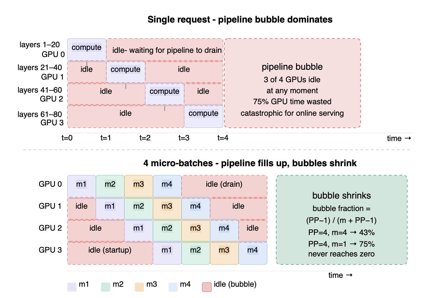
Figure 5.2 - Pipeline parallelism (PP=4): the bubble problem
Top: a single request enters the pipeline - GPU 0 computes its layers and passes activations down, then sits idle for 3 time steps while GPUs 1, 2, and 3 process sequentially. At any given moment 3 of 4 GPUs are idle - 75% of GPU time wasted. Bottom: 4 micro-batches fill the pipeline - while GPU 3 processes m1, GPU 2 processes m2, GPU 1 processes m3, and GPU 0 processes m4 simultaneously. Bubbles shrink to the startup and drain edges. But the bubble fraction formula (PP−1)/(m + PP−1) shows it never reaches zero: PP=4 with 4 micro-batches still wastes 43% of GPU time. This is why PP is reserved for models too large to fit within a single NVLink domain - for online serving with variable input lengths, TP within a node is always preferred.
Pipeline parallelism is best suited for offline batch inference where you can keep the pipeline full with large batches, and where per-request latency matters less than aggregate throughput. For latency-sensitive online serving with variable input lengths - which LLM workloads almost always have - TP is generally preferred within a node, with PP reserved for cases where the model simply cannot fit within a single node's NVLink domain.
When a model exceeds a single node's NVLink domain entirely, neither TP nor PP alone is sufficient - which is where the two strategies are combined, covered next.
5.3 Data Parallelism: The Cleanest Scaling Strategy
Tensor and pipeline parallelism both solve the same class of problem - fitting a model that is too large or too slow for one GPU. Data parallelism solves a completely different problem: what do you do when your single instance is already well-configured but you simply need more of them?
Data parallelism runs N completely independent model replicas across N GPU groups. Each replica processes its own request stream with no inter-replica communication during inference - no all-reduce, no activation transfer, no coordination overhead of any kind between replicas at the compute level. A load balancer distributes incoming requests across replicas. Doubling the replica count doubles RPS capacity with linear cost scaling and zero latency overhead. The only hard constraint is that each GPU group must hold a complete model copy - DP does not reduce per-instance memory requirements.
This simplicity is real but it comes with a few operational nuances that production deployments must handle explicitly.
Load balancing is not round-robin. LLM requests have wildly different token lengths and therefore wildly different latency profiles. Naive round-robin routing ignores replica load state - a long-context request routed to an already-loaded replica causes head-of-line blocking that degrades the entire replica's queue. Production deployments use latency-aware or queue-depth-aware routing. The load balancer is a first-class component of the DP architecture, not an afterthought.
Cold start latency scales with model size. Each replica is a full model copy. At 70B FP8 that is 70 GB per replica - loading from NVMe to GPU before the replica can serve its first request. Autoscaling response time for DP is directly proportional to model size, which means large models have slow autoscaling. Size down aggressively with quantization before scaling out with DP, and pre-warm replicas where possible rather than spinning them up on-demand.
Multi-turn sessions require sticky routing. Each replica maintains its own independent KV cache. A multi-turn conversation where subsequent requests land on different replicas will find no cached KV state from prior turns - the model effectively loses context. Production deployments either implement sticky routing to pin sessions to replicas, or accept the KV cache miss cost and recompute context on each turn. The choice has both latency and cost implications.
Rolling deployments require replica-level coordination. Replicas share the same weights at any given time, but updating model versions across a fleet requires careful replica management - canary deployments, A/B version splits, and graceful drains all need orchestration at the replica level. DP replicas are independent at the compute level but not at the operations level.
The production scaling pattern that emerges from all of this: use TP within a node to fit the model and meet latency SLOs, then scale horizontally with DP across nodes to meet throughput requirements. TP handles the memory and latency problem. DP handles the capacity problem. These two levers compose cleanly at the architecture level - the operational complexity lives in the DP layer, not the TP layer.
The three strategies above apply to dense transformer models - every parameter participates in every forward pass. Mixture-of-Experts architectures break that assumption entirely, and when they do, a fourth parallelism strategy becomes not just useful but necessary.
5.4 Expert Parallelism: For MoE Architectures
In every parallelism strategy covered so far, every parameter participates in every forward pass. MoE architectures break this assumption - and when they do, the economics of inference change fundamentally.
Mixture-of-Experts models - DeepSeek-V3, Mixtral 8×7B, Qwen-MoE - have changed what "model size" means for inference. Each token is routed to a small subset of specialist feed-forward layers called experts, with the rest unused for that token. Total parameter count is large; active parameter count per forward pass is much smaller. DeepSeek-V3 has 671B total parameters but activates only ~37B per token - you store a 671B model but pay compute cost closer to a 37B model on every forward pass. The economic leverage is real, but it comes with a set of engineering problems that dense parallelism strategies do not have.
How EP works. Expert Parallelism distributes different experts across different GPUs. When a token is routed to Expert 7, it is dispatched via an all-to-all communication to the GPU hosting Expert 7's weights, computed there, and the result returned via a second all-to-all. This allows serving models with hundreds of billions of parameters at a fraction of the compute cost implied by their total size - because most of those parameters are inactive for any given token.
The engineering challenge is routing overhead: tokens must be dispatched to the correct expert GPU, which requires fast all-to-all communication across the expert GPU pool. Wide Expert Parallelism (Wide-EP), implemented in TensorRT-LLM, scales this to very large expert pools and has demonstrated 1.8x higher per-GPU throughput than smaller EP setups on an NVL72 system. Wide-EP works because NVL72's 72-GPU NVLink domain provides the all-to-all bandwidth density needed to keep routing latency from dominating - on systems without this interconnect density, Wide-EP's gains shrink significantly. For MoE models at scale, EP is not optional - it is the mechanism that makes the economics viable.
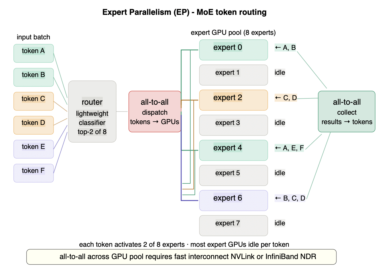
Figure 5.4 - Expert parallelism: MoE token routing across GPU pool
Each token is scored by a lightweight router and dispatched to its top-2 experts out of the full expert pool. An all-to-all communication sends each token to its assigned expert GPUs, each expert computes independently, and a second all-to-all collects results back to the originating tokens. At any given moment most expert GPUs are idle - for DeepSeek-V3 with 256 experts, each token activates only 2, leaving 254 inactive. The economic insight: you store 671B parameters but pay compute cost for only ~37B active parameters per token. The contrast with TP is fundamental - TP broadcasts every token to every GPU; EP routes each token to a small subset. The engineering challenge is the all-to-all communication pattern, which requires fast interconnect (NVLink or InfiniBand NDR) and careful load balancing to avoid hot experts that receive disproportionate token traffic.
The mechanism is straightforward. The production engineering challenges are not.
Memory sizing is not as simple as "671B divided by GPU count." The active parameter framing is useful for compute cost estimation but misleading for memory sizing. You still store all 671B parameters - EP distributes them across GPUs, it does not eliminate them. Additionally, most production MoE architectures include shared experts that run on every token regardless of routing. DeepSeek-V3 has shared experts that function as a dense component sitting alongside the sparse routed component. Memory budgeting must account for both the routed experts on each GPU and the shared expert weights that every GPU carries.
EP and TP are almost always combined. For large MoE models, individual expert weights may not fit on a single GPU, or the TP degree needed to meet latency SLOs requires splitting within each expert. Production deployments combine EP to distribute experts across GPUs with TP within each expert group. Sizing requires deciding both the EP degree - how many GPU groups to distribute experts across - and the TP degree within each group. These interact: higher EP degree reduces per-GPU expert memory but increases all-to-all communication surface; higher TP degree reduces per-GPU expert compute time but adds all-reduce overhead within each expert group.
The expert load imbalance problem is the critical production constraint. EP throughput is bounded by the busiest expert, not the average. If your workload causes one expert to receive 3× the average token traffic - which happens regularly due to training distribution biases - the entire EP group runs at roughly one-third of theoretical throughput regardless of how idle the other GPUs are. This is not a theoretical concern: in production deployments, unmeasured expert utilization distributions are the most common source of EP underperformance. Before committing to an EP configuration, measure your actual expert activation distribution on your specific workload. Production EP deployments mitigate this through two mechanisms: a capacity factor at the router level that caps how many tokens any single expert can receive per batch - forcing overflow tokens to a backup expert rather than stalling the pipeline - and expert-aware load balancing in the serving framework that monitors utilization in real time and rebalances routing weights when hot spots emerge. Neither mechanism eliminates imbalance entirely, but together they keep it manageable. The practical takeaway: always set a capacity factor above 1.0 in your serving configuration, and monitor per-expert token counts as a production metric from day one.
Expert overflow causes silent quality degradation. Each expert has a fixed capacity - a maximum number of tokens it can process per forward pass. When routing sends more tokens to an expert than its capacity allows, the overflow tokens are either dropped or rerouted to a backup expert. This does not throw an error - the model silently produces degraded output for overflow tokens. Setting the expert capacity factor too low to save memory is a common mistake that produces quality regressions that are difficult to attribute. In production, always monitor expert overflow rates as a first-class metric alongside throughput and latency.
EP adds latency that does not compress well. The all-to-all communication at each MoE layer is a synchronization barrier - every token must wait for the slowest expert to finish before computation proceeds to the next layer. Unlike the TP all-reduce which can be partially overlapped with computation, the EP all-to-all is harder to hide. At large EP degrees on slower interconnects, this latency accumulates across MoE layers and adds meaningfully to TTFT. EP is primarily a throughput optimization - it makes large MoE models economically viable at scale - but it is not a latency optimization. For strict TTFT SLOs, EP degree should be kept as low as memory constraints allow.
5.5 How Production Systems Combine These Strategies
The four strategies are building blocks. Production systems assemble them based on three independent constraints: does the model fit on one GPU, does it fit within one node, and is it a dense or MoE architecture? Each combination below addresses a specific combination of those constraints. No large-scale production deployment uses a single parallelism strategy in isolation. The standard patterns:
| Combination | When Used | What Each Strategy Does | Key Constraint |
|---|---|---|---|
| TP × DP | Standard production setup (e.g., 70B-class models) | TP fits the model within a node and reduces latency. DP replicates across nodes to scale throughput (RPS) | Memory and latency handled by TP. Capacity scaling via DP. |
| TP × PP | Model too large to fit within a single node even with maximum TP | TP distributes compute within a node. PP splits layers across nodes | Inter-node bandwidth (InfiniBand / RoCE) becomes the bottleneck |
| TP × DP × EP | Large-scale MoE serving | TP handles attention layers within each node. EP distributes experts across GPUs. DP scales replicas for throughput | All-to-all communication for expert routing plus overall system load balance. |
The decision logic is simpler than it looks. Start with a single GPU. If the model does not fit, apply TP within the node. If it still does not fit, add PP across nodes. Once the per-instance configuration is right, scale horizontally with DP. If you are serving MoE, layer EP on top of TP for the expert layers. You are almost never choosing between these strategies - you are stacking them in the right order for your specific constraints.
5.6 The Interconnect Is Not a Detail
Every combination in the previous section has one variable that determines whether the theoretical performance is actually achievable: the interconnect fabric between GPUs.
The interconnect landscape - which technology serves which transfer path
Different parallelism strategies generate fundamentally different data movement patterns, and each pattern has its own physical interconnect. Understanding which technology applies where is the prerequisite for making any inter-node procurement decision.
| Transfer path | What moves | Technology | Typical bandwidth |
|---|---|---|---|
| GPU ↔ GPU (same node) | Activations, all-reduce gradients (TP) | NVLink (NVSwitch on DGX/HGX) | ~900 GB/s bidirectional |
| GPU ↔ CPU DRAM (same node) | KV cache swap, model checkpoint | PCIe Gen4/Gen5 | 64-128 GB/s |
| GPU ↔ NVMe (same node) | Model weight loading at cold start | PCIe Gen4/Gen5 via NVMe controller | ~12.5 GB/s |
| Node ↔ Node (inter-node) | PP activations, EP all-to-all, KV transfer in disaggregation | InfiniBand NDR or RoCE v2 | 25-50 GB/s per link |
| Node ↔ Object storage | Model artifact loading (S3, GCS) | Ethernet (10/25/100 GbE) | 1-12 GB/s effective |
The table makes the scoping explicit: NVLink solves intra-node TP. InfiniBand or RoCE solve inter-node PP and EP. PCIe solves CPU-GPU and NVMe transfers. These are not competing technologies - they are complementary layers in the same stack, each sized for a different bottleneck.
Intra-node: NVLink vs PCIe
The interconnect is the most common reason TP deployments underperform their theoretical speedup. Teams that benchmark TP=4 on PCIe and see disappointing latency frequently conclude that their model does not parallelize well - when the actual problem is that roughly 25% of every step is spent on communication rather than compute. NVLink does not just improve TP performance. It determines whether TP above 2 is worth deploying at all.
Within a DGX or HGX H100 node, NVLink provides ~900 GB/s of GPU-to-GPU bandwidth. PCIe Gen5 provides ~128 GB/s per x16 link - a 7× difference that is not marginal. At TP=2, PCIe overhead sits around 8% of step time - uncomfortable but manageable. At TP=4, it reaches ~25%. At TP=8, it exceeds 38% - more than a third of every step spent moving data rather than computing. The latency benefit of higher parallelism is progressively eroded until at TP=8 on PCIe the communication overhead effectively negates the compute saving.
The practical decision rule: TP=2 is acceptable on PCIe when NVLink is unavailable. TP=4 on PCIe should be benchmarked carefully against TP=2 before committing - the theoretical 2× compute benefit rarely survives the communication overhead in practice. TP=8 on PCIe is almost never worth deploying except for the most compute-bound prefill workloads where the arithmetic intensity is high enough to tolerate the communication tax.
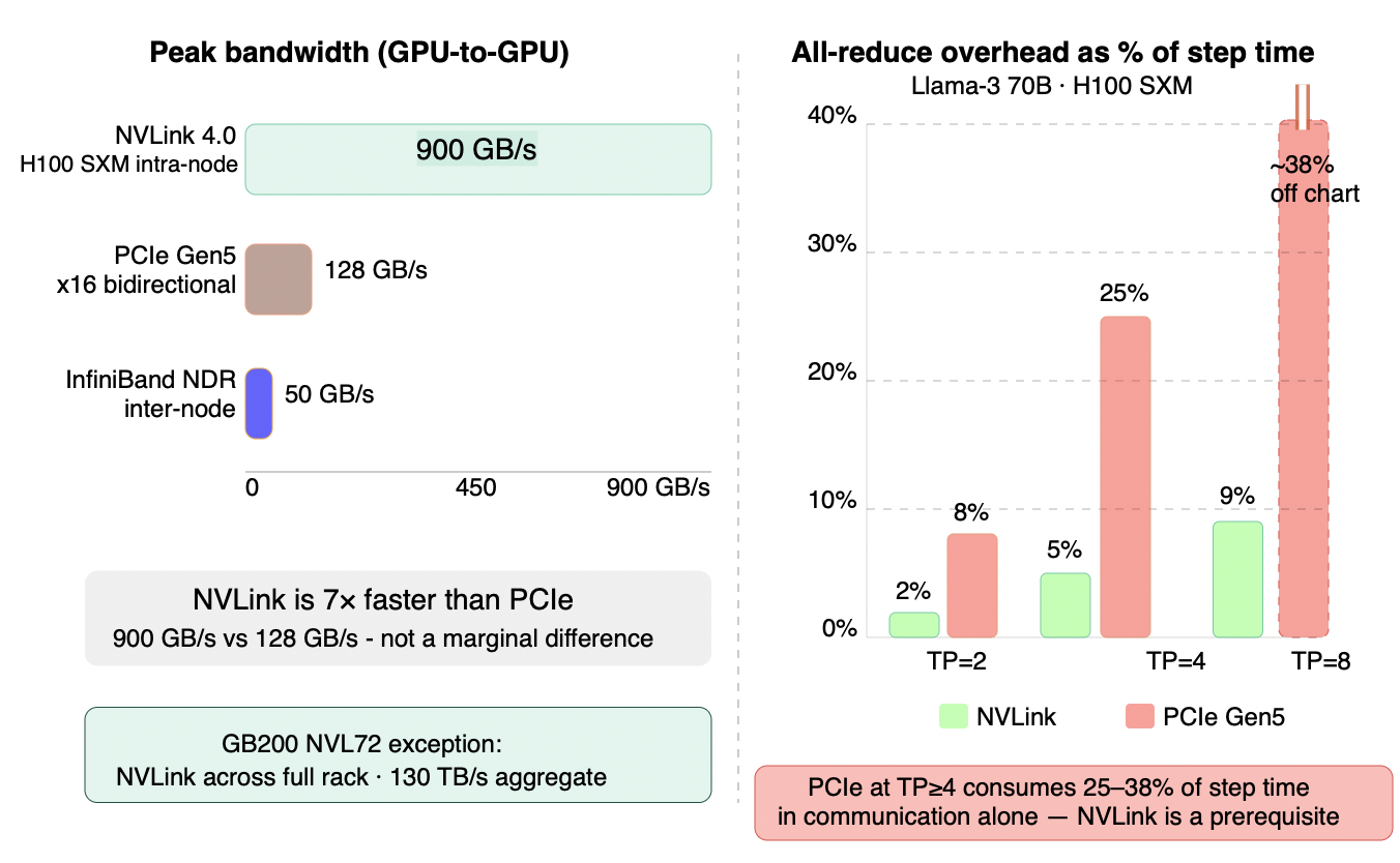
Figure 5.6 - NVLink vs PCIe: interconnect bandwidth and all-reduce overhead
Left: NVLink's 900 GB/s intra-node bandwidth is 7× faster than PCIe Gen5's 128 GB/s - not a marginal difference. InfiniBand NDR at ~50 GB/s governs inter-node communication for PP. Right: the consequence at different TP degrees. On NVLink, all-reduce overhead stays at 2-9% of step time across TP=2 through TP=8 - acceptable at any TP degree. On PCIe, overhead is already 8% at TP=2 and reaches ~25% at TP=4 - a quarter of every step spent on communication rather than compute. At TP=8 on PCIe the overhead exceeds 38%, effectively negating the latency benefit of higher parallelism. NVLink is a prerequisite for deployments with TP > 2.
Inter-node: InfiniBand NDR vs RoCE v2
For multi-node PP and EP deployments, inter-node bandwidth determines whether activation transfers and all-to-all communication remain manageable or dominate step time.
InfiniBand NDR (~50 GB/s per link) is purpose-built for GPU-to-GPU RDMA with hardware-managed congestion control. It works reliably out of the box for PP and EP traffic patterns at a significant cost premium over Ethernet.
RoCE v2 delivers comparable bandwidth over standard 100/400 GbE infrastructure at lower cost, but requires correct network configuration to behave reliably under load. When misconfigured, tail latency spikes under congestion and PP bubble fractions grow - eroding the parallelism gains the interconnect was supposed to enable.
Decision rule: use InfiniBand NDR for new multi-node deployments where reliability matters and budget allows. Use RoCE v2 where existing GbE infrastructure is in place and your networking team has RDMA experience. Either way, validate inter-node bandwidth under realistic PP or EP load before committing to an architecture that depends on it.
With the parallelism configuration and interconnect fabric determined, the unit of compute is defined. The next question is how to saturate it - which is the batching strategy covered in Section 6.