3 · The Roofline Model: Why Prefill and Decode Differ
Most discussions of LLM inference treat it as a single workload with a single performance curve. This is the root cause of a class of sizing mistakes that no amount of GPU provisioning can fix - because they stem from a mismatch between what the hardware is good at and what the workload demands of it. A team that sizes for throughput on a decode-dominated workload and buys H100s for their TFLOPS will be disappointed - the bottleneck was never compute. More TFLOPS do not help when the chip is starving for memory bandwidth.
LLM inference is two distinct computational workloads running sequentially on the same hardware. They have different arithmetic profiles, hit different hardware limits, and respond to different optimizations. Understanding why requires one foundational concept: arithmetic intensity.
3.1 Arithmetic Intensity: The Number That Determines Your Bottleneck
Every GPU has two hard performance ceilings. The first is peak compute throughput, measured in TFLOPS - how many floating point operations the chip can execute per second. The second is peak memory bandwidth, measured in TB/s - how fast data can move between HBM (the high-bandwidth memory on the GPU) and the compute units that actually do the math.
Arithmetic intensity captures the ratio between these two demands for any given operation:
Arithmetic intensity = TFLOPs required / bytes of memory moved
When arithmetic intensity is high - many computations per byte fetched from memory - the operation is compute-bound: it saturates the TFLOPS ceiling before it saturates memory bandwidth. When arithmetic intensity is low - few computations per byte - the operation is memory-bandwidth-bound: the compute units sit idle waiting for data that memory cannot deliver fast enough.
The ridge point of the roofline is the arithmetic intensity at which both ceilings are hit simultaneously:
Ridge point = peak TFLOPS / peak HBM bandwidth (in FLOP/byte)
For an H100 SXM: approximately 989 TFLOPS (TF32) / 3.35 TB/s = roughly 295 FLOP/byte. Any operation above this threshold is compute-bound. Below it, memory bandwidth is the constraint. This single number is why prefill and decode require fundamentally different hardware thinking.
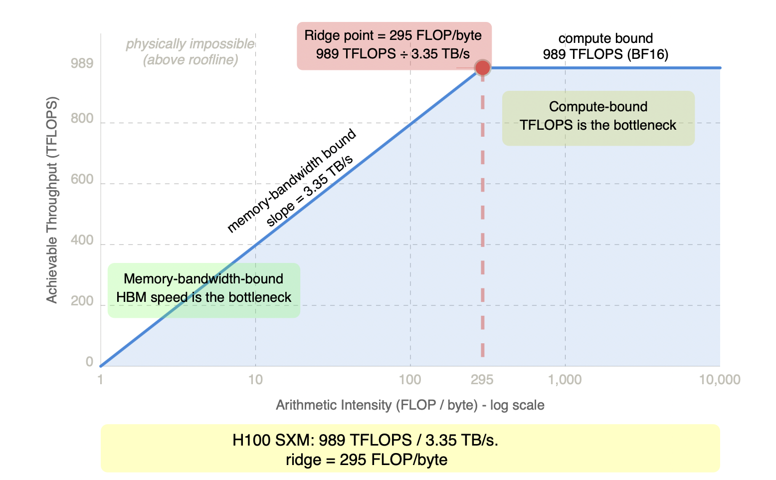
Figure 3.1 - The roofline model for H100 SXM
Every GPU operation is bounded by one of two hard ceilings. Below the ridge point (295 FLOP/byte on H100 SXM), memory bandwidth is exhausted before compute - adding more TFLOPS does nothing. Above it, compute is exhausted before memory bandwidth - faster HBM does nothing. The roofline is not a guideline: no software optimization can push an operation above it. Only restructuring the computation (e.g. larger batch sizes) or changing the hardware can shift where an operation sits on this chart. The next two sections show exactly where prefill and decode land.
The ridge point is the dividing line. The next two sections show exactly where prefill and decode land relative to it - and why they land on opposite sides.
3.2 Prefill Is Compute-Bound
Prefill lands well above the ridge point. Here is why. During prefill, the model processes all input tokens simultaneously in a single parallel forward pass. This is structurally a large matrix multiplication: the input token matrix (shape: sequence_length × hidden_dimension) is multiplied against the weight matrices in each transformer layer. Matrix multiplications have high arithmetic intensity because the same weight values are reused across many token positions in the same operation - the compute-to-memory-access ratio is high.
The practical consequence is significant: prefill saturates GPU compute even at batch size 1. A single request with a 4K-token prompt will fully occupy the CUDA cores of an H100. Adding more concurrent prefill requests to the same batch does not meaningfully increase per-request throughput - the compute ceiling is already being hit. What you gain from batching prefill is amortization of the fixed overhead per forward pass, not escape from the bottleneck. This means prefill throughput scales with TFLOPS, not with batching strategy. The lever for higher prefill RPS is faster compute - either a higher-TFLOPS GPU or, for very large deployments, dedicated prefill instances separated from decode. This is the architectural motivation for prefill-decode disaggregation, covered in subsequent sections.
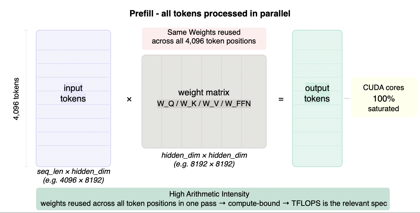
Figure 3.2 - Prefill: large matrix × large matrix
During prefill, all input tokens are processed simultaneously - a [seq_len × hidden_dim] matrix multiplied against each weight matrix in the layer stack. The same weights are reused across every token position in a single pass, producing high arithmetic intensity. CUDA cores stay fully occupied. The bottleneck is compute, not memory.
For prefill-dominated workloads - RAG pipelines processing long retrieved contexts, document summarization, legal or medical record analysis - the relevant GPU specification is TFLOPS. An H100 SXM at 989 TFLOPS BF16 dense completes the same prefill roughly 3× faster than an A100 at 312 TFLOPS BF16 - the memory bandwidth difference between them is proportionally much smaller and largely irrelevant for this workload type. More compute throughput means faster prefill, lower TTFT, higher prefill RPS. Memory bandwidth matters less because the arithmetic intensity of large matrix multiplications keeps the compute units occupied.
3.3 Decode Is Memory-Bandwidth-Bound
Decode is structurally the opposite problem. If prefill is the GPU doing too much work per byte, decode is the GPU doing too little - starved for data rather than overwhelmed by computation. Each decode step generates exactly one new token. To do so, the model must load the full weight matrix for every transformer layer from HBM into on-chip SRAM, perform a small matrix-vector multiplication (one token position against the full weight matrix), and discard the intermediate activations while updating the KV cache. Then repeat for the next layer.
The arithmetic intensity of this operation is extremely low. You are moving hundreds of gigabytes of weight data through the memory bus to perform a trivially small amount of arithmetic on it - one token's worth of computation per multi-gigabyte weight matrix. The compute units finish their work almost instantly and then wait for the next chunk of weights to arrive from HBM. The GPU is not doing math most of the time. It is waiting for memory.
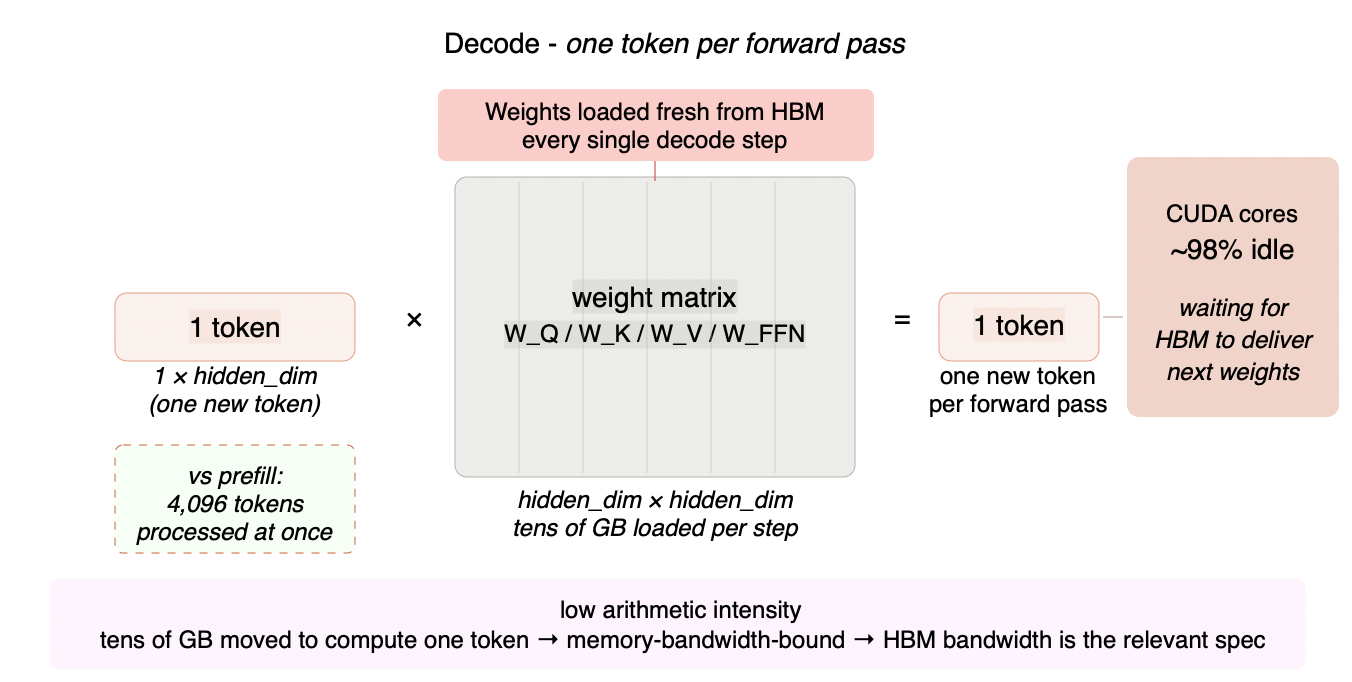
Figure 3.3 - Decode: large matrix × single vector
During each decode step, only one new token is generated. The full weight matrix - tens of gigabytes - is loaded fresh from HBM on every step, but multiplied against a single token vector. The arithmetic intensity collapses to near zero. CUDA cores finish their work almost instantly and sit idle while the memory bus delivers the next chunk of weights. The bottleneck is HBM bandwidth, not compute.
SARATHI's (chunks prefills and co-batches them with decodes so decodes piggyback on prefill compute) profiling data makes this concrete: at batch size 1, decode per-token cost can be up to 200× higher than prefill per-token cost on the same hardware. The weights do not change between a prefill step and a decode step - the computational structure does, and that structural change moves the operation from well above the roofline ridge point to well below it. This is not an inefficiency that can be tuned away. It is a direct consequence of arithmetic intensity collapsing from ~1,000 FLOP/byte during prefill to ~2 FLOP/byte during decode - a 500× difference in computational density on the same hardware running the same model.
For decode-dominated workloads - code generation, long-form content creation, extended reasoning chains - the relevant GPU specification is HBM bandwidth, not TFLOPS. The AMD MI300X at 5.3 TB/s and 192GB capacity delivers meaningfully better decode throughput than the H100 SXM at 3.35 TB/s and 80GB capacity for the same model, despite the H100 having superior raw compute. The comparison reverses for prefill-heavy workloads where TFLOPS dominates. This is not a marketing distinction - it is a direct consequence of where each workload sits relative to the roofline ridge point.
The roofline chart makes the contrast unavoidable. Placing both operating points on the same axes shows not just that prefill and decode are different - it shows how different, and why the gap cannot be closed by any single hardware choice or software optimization.
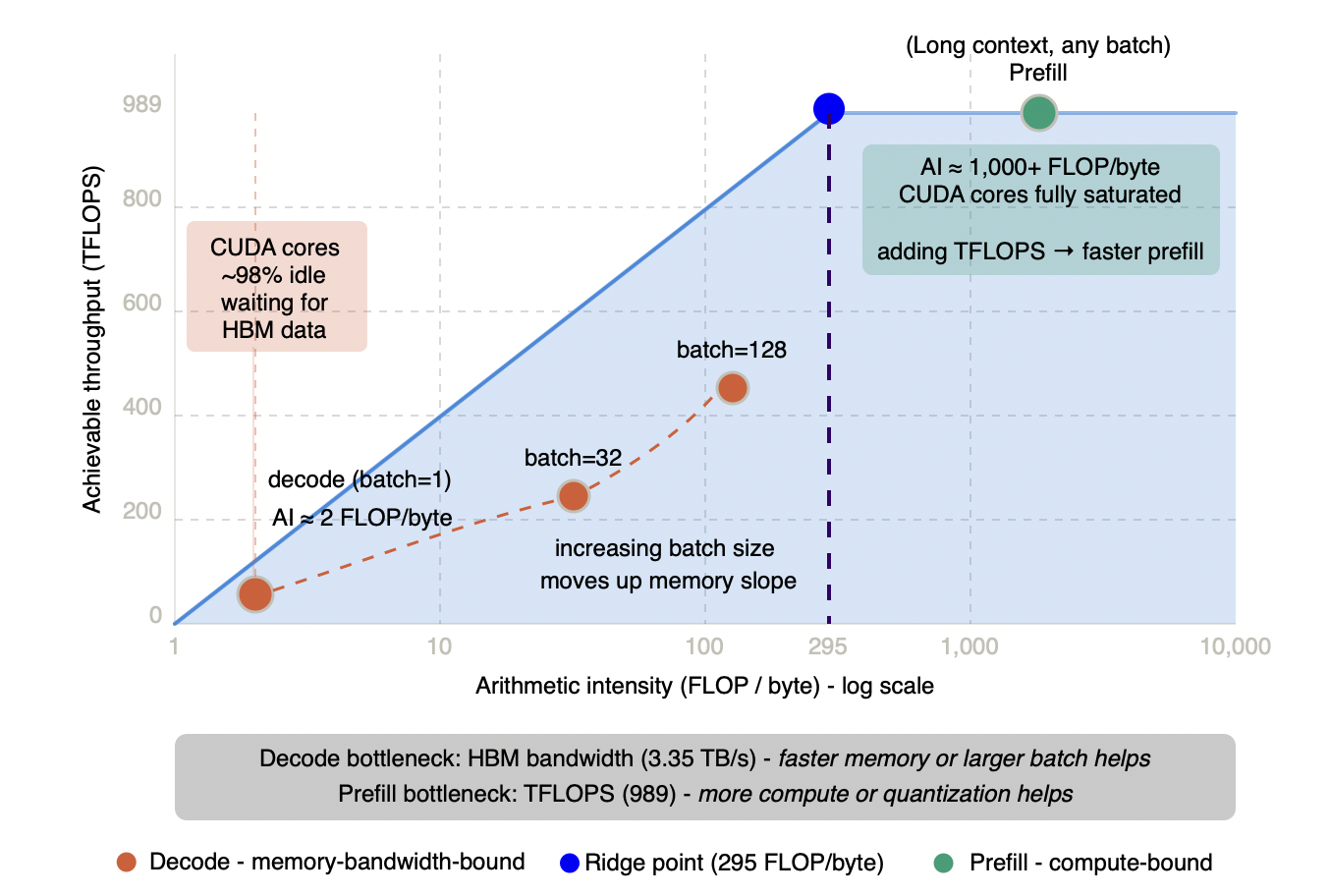
Figure 3.3.2 - Prefill and decode operating points on the H100 roofline
Prefill sits at the compute ceiling - processing all prompt tokens in parallel produces arithmetic intensity well above 295 FLOP/byte, fully saturating CUDA cores regardless of batch size. Decode at batch=1 sits deep in the memory-bandwidth-bound region at roughly 2 FLOP/byte, leaving CUDA cores ~98% idle while the memory bus works at capacity. Larger batch sizes move decode up the memory-bound slope - but never past the ridge point into compute-bound territory. The two phases are not variations of the same problem. They are different problems on the same hardware, and they respond to different solutions.
GPU selection for a mixed workload is therefore not a single decision. It is a weighted average of where your traffic sits on the prefill-decode spectrum. A RAG pipeline spending 80% of compute time in prefill should optimize for TFLOPS. A code generation service spending 80% of compute time in decode should optimize for HBM bandwidth. Buying the wrong GPU for your workload mix is a sizing mistake that no software configuration can compensate for. Batch size is the one lever that moves decode's operating point up the memory-bound slope - and it is significant enough to warrant its own section.
3.4 Batch Size Is the Primary Lever for Decode Efficiency
Batch size is the one variable that directly improves decode's arithmetic intensity - and therefore the one variable that moves its operating point up the memory-bound slope toward the roofline.
The mechanism is straightforward. Every decode step requires loading the full weight matrices for every transformer layer from HBM - a fixed bandwidth cost paid regardless of how many requests are being served simultaneously. At batch size 1, that cost buys one token of output. At batch size 64, the identical memory transfer produces 64 tokens of output. The arithmetic intensity scales linearly with batch size because the compute work multiplies while the memory access cost stays constant. This is the fundamental reason batching matters for decode in a way it does not for prefill: you are spreading a fixed bandwidth tax across more useful work.
The practical consequence is substantial. At batch=1 on a Llama-3 70B FP8 on H100, decode throughput is approximately 80 tokens per second - the memory bus is working at capacity but producing almost nothing because the compute units are nearly idle. At batch=128, throughput reaches approximately 4,700 tokens per second - roughly 60× higher - with the same weight-loading cost per step. The ceiling is a hardware limit, not a configuration limit. Once HBM bandwidth is fully saturated, no software optimization pushes the curve higher.
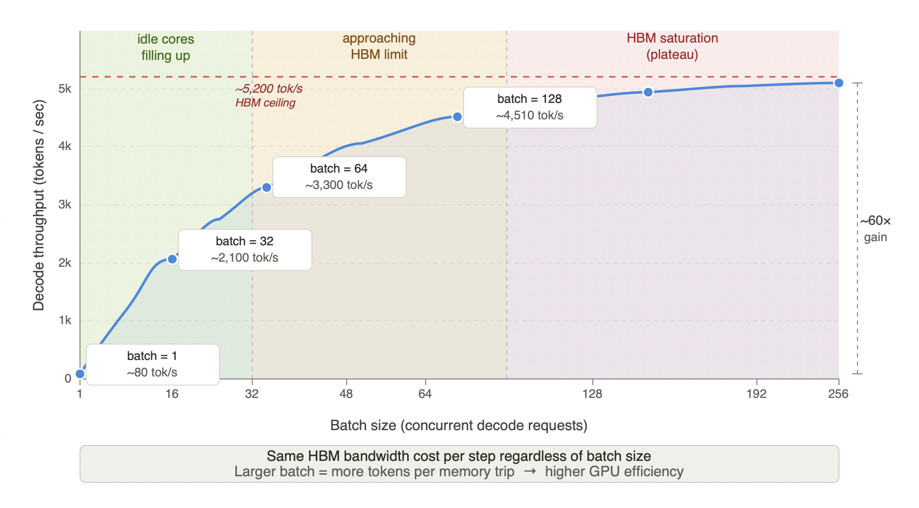
Figure 3.4 - Decode throughput vs batch size (Llama-3 70B FP8, H100 SXM)
At batch=1, the memory bus is already working at capacity - loading the full weight matrices every decode step - but producing only ~80 tokens per second because the compute units are nearly idle. Each additional request in the batch amortizes that same fixed memory cost across more simultaneous token generations, putting idle CUDA cores to work. Throughput scales near-linearly through the green zone as idle compute fills up, bends through the amber zone as the memory bus approaches saturation, and plateaus in the red zone when HBM bandwidth is fully exhausted - a hardware ceiling no software optimization can push past. At batch=128 throughput reaches ~4,510 tok/s, roughly 60× higher than batch=1 for identical hardware cost per step. The plateau makes the constraint explicit: beyond ~192 concurrent requests, adding more users yields diminishing returns until more GPUs or faster HBM are introduced. This ~60× gap is why continuous batching is not optional for production deployments - a system serving requests one at a time is paying full HBM bandwidth cost for a fraction of the achievable output.
This asymmetry does not apply to prefill. Prefill already saturates compute at batch size 1 - processing all input tokens simultaneously naturally fills the CUDA cores. Adding concurrent prefill requests does not find idle compute capacity; it forces requests to share the same ceiling, increasing TTFT without a proportional throughput gain. The roofline positions of the two phases are fixed by their arithmetic intensity, and batching only helps the phase that has idle resources to fill. For decode, those resources are the compute units. For prefill, there are none to recover. This structural difference is the architectural motivation for separating them entirely - covered in subsequent sections.
3.5 Hardware Strategy: The Roofline Trade-off
Batch size moves the operating point up the memory-bound slope - but it cannot change which side of the ridge point a workload sits on. That is a hardware decision, and the roofline model makes it precise.
A fleet optimized for prefill needs TFLOPS. The H100 SXM at 989 TFLOPS TF32 (1,979 TFLOPS BF16 with sparsity) and the B200 at 2,250 TFLOPS BF16 dense (4,500 TFLOPS with sparsity) are the right choices for RAG pipelines, document summarization, and any workload where input context is long and output is short. Memory bandwidth is secondary - the arithmetic intensity of large matrix multiplications keeps the compute units saturated regardless.
A fleet optimized for decode needs HBM bandwidth. The AMD MI300X at 5.3 TB/s versus the H100 SXM at 3.35 TB/s delivers approximately 58% higher peak memory bandwidth - a direct consequence of the memory bus being the binding constraint for decode. The MI300X also carries 192 GB of HBM versus 80 GB on the H100, meaning larger models or higher KV cache budgets without tensor parallelism. NVIDIA's own H200 at 4.8 TB/s and 141 GB HBM3e partially closes this gap and is the current recommended Hopper-generation upgrade for decode-heavy workloads. For code generation, extended reasoning, and chat workloads where output length dominates, optimizing for bandwidth per dollar rather than TFLOPS per dollar is the correct framing.
For mixed workloads, neither GPU is unambiguously correct. The right answer is to measure your actual input-to-output length ratio under production traffic, compute the fraction of wall-clock time spent in prefill versus decode, and weight the hardware comparison accordingly. Headline throughput benchmarks are almost always measured under prefill-favorable conditions and will overstate performance on decode-heavy workloads.
The architectural implication. The roofline analysis exposes a fundamental tension: any single GPU fleet is a compromise between two workloads with opposite hardware requirements. The resolution is disaggregated prefill-decode architecture - separate GPU pools for each phase, each sized and configured for its specific bottleneck. This is covered in the disaggregation section later in this guide.
Quantization affects the two phases differently. Reducing weight precision from FP16 to FP8 or INT8 halves the bytes transferred per weight matrix load. For decode - where the bottleneck is memory bandwidth - this directly raises the throughput ceiling: the same HBM bandwidth now moves twice as many weight values per second, and FP8 decode throughput approaches 2× FP16 at bandwidth saturation. For prefill - where the bottleneck is compute - the same quantization saves VRAM and reduces weight-loading time but does not increase TFLOPS. The speedup for prefill comes primarily from fitting larger batches or longer contexts into the same memory budget, not from hitting a higher compute ceiling. This asymmetry means quantization decisions cannot be evaluated on a single throughput number - they must be evaluated separately for each phase. Section 4 covers quantization strategy in full.